Conditional formatting is a super useful technique for formatting cells in your Google Sheets based on whether they meet certain conditions.
In this post, you’ll learn how to apply conditional formatting across an entire row of data in Google Sheets.
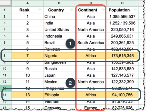
For example, if the continent is “Africa” in column C, you can apply the background formatting to the entire row (as shown by 1 and 2):
A template with all these examples is available at the end of this post.
How To Apply Conditional Formatting Across An Entire Row
It’s actually relatively straightforward once you know the technique using the $ sign (Step 5).
Step 1. Highlight the data range you want to format
The first step is to highlight the range of data that you want to apply your conditional formatting to. In this case, I’ve selected:
A2:C13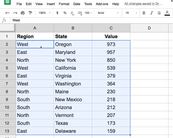
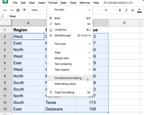
Step 2. Choose Format > Conditional formatting… in the top menu
Open the conditional format editing side-pane, shown in this image, by choosing Format > Conditional formatting… from the top menu:
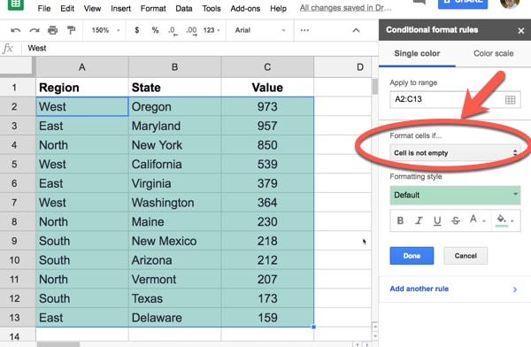
Step 3. Choose “Custom formula is” rule
Google Sheets will default to applying the “Cell is not empty” rule, but we don’t want this here.
Click on the “Cell is not empty” to open the drop-down menu:
Scroll down to the end of the items in the drop-down list and choose “Custom formula is”. This will add a new input box in the Format cells if section of your editor:
Step 4. Enter your formula, using the $ sign to lock your column reference
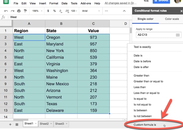
In this example, I want to highlight all the rows of data that have “West” in column A. In this new input box, enter the custom formula:
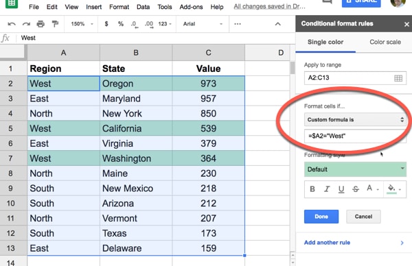
The key point to understand is that you lock the column you want to base your conditional formatting on by adding a $ (dollar sign) to the column reference.
I start inputting the first cell of my highlighted range:
= A2It’s really important that the row here matches the first row of your highlighted range (e.g. if your data is A10:C50 then your conditional formatting rule start with A10 too).
Then I add the $ (dollar sign) in front of the A only:
= $A2Then I add the test condition, in this case whether the cell equals “West”:
= $A2 = "West"As the conditional formatting test is applied across each row, the value from the first cell in column A is used in the check.
To learn more about using the $ sign and understand relative and absolute references, have a read of this post: How To Use Google Sheets: A Beginner’s Guide
More Examples Of Conditional Formatting Across An Entire Row
Based on a threshold value
This is a super useful application of this technique, to dynamically highlight rows of data in your tables where a value exceeds some threshold.
In this example, I’ve highlighted all of the students who scored less than 60 in class, using this formula in the custom formula field:
= $C2 < 60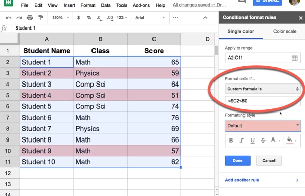
Based on checkboxes
Google Sheets checkboxes are super useful. If you haven't heard of them or used them yet, you're missing out.
When a checkbox is selected it has the value TRUE, and when it is not selected the cell has the value FALSE. So we can use that property in our custom formula:
= $B2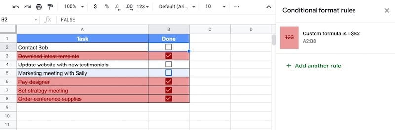
Multi-Condition Examples
AND Example: Highlight Whole Row When Two Conditions Are Both True
Often we want to highlight based on two conditions. In this example, we'll see how to highlight the entire row when both conditions are true.
Here, we want to highlight all rows with "Apartment" in column B and "Buyer" in column D.
We use an AND Function to do this.
Highlight the dataset and add this conditional formatting custom formula:
=AND($B1="Apartment",$D1="Buyer")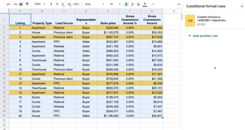
OR Example: Highlight Whole Row When Condition A or Condition B Are True
This is similar to the previous example, but now we want to highlight rows where either (or both) of the conditions are true.
We use an OR Function to do this.
Conditions In Same Column
Firstly, let's see an example where the two conditions can exist in the same column.
We want to highlight all rows with "House" in column B or "Townhouse" in column B. Notice both conditions in column B.
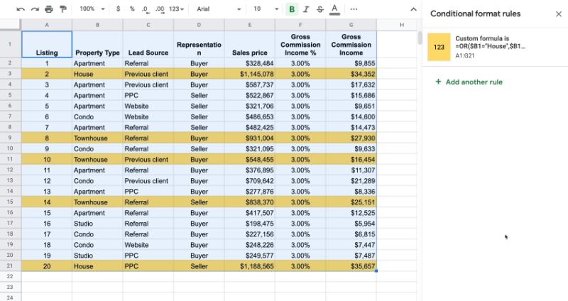
This is the conditional formatting custom formula we use:
=OR($B1="House",$B1="Townhouse")Conditions In Different Columns
This time, imagine the two conditions exist in different columns.
For example, suppose we want to highlight all rows with "House" in column B or sales price > $700,000 in column E.
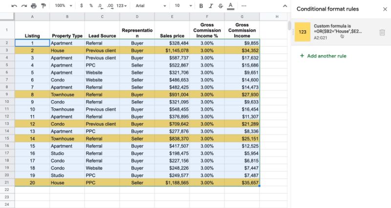
Use this rule to achieve this:
=OR($B2="House",$E2>700000)*** Notice how the rule starts on row 2 this time and is only applied to the data but not the header row. That's because the condition $E1 > 700000 evaluates to TRUE for the text heading (bizarre!), which we want to avoid.
Three Condition Example
Suppose we want to check for a third condition...
We combine an AND function with an OR function and use brackets to determine the precedence (i.e. the order) that the tests are carried out.
Consider this example:
=OR($B1="House",AND(ISNUMBER($E1),$E1>700000))The rule will highlight the row when there is either:
- "House" in column B, OR
- Column E is a number AND it's greater than $700,000
The two conditions on column E must both be TRUE for the AND to evaluate to TRUE.
This rule is another way to solve the header issue in the previous example.
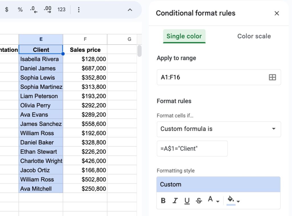
How To Apply Conditional Formatting to an Entire Column
We use the same idea as with the examples above, but we lock the formula to a specific row instead of a column.
So the formula to apply conditional formatting to entire columns is:
=A$1="Client"This rule checks for client in row 1 and if it finds client, the formatting is applied to the whole of that column:
Conditional Formatting Template
Click here to open a view-only copy >>
Feel free to make a copy: File > Make a copy...
If you can't access the template, it might be because of your organization's Google Workspace settings. If you right-click the link and open it in an Incognito window you'll be able to see it.
 💡 Learn more
Check out my beginner course and master key techniques to become confident with Google Sheets: Google Sheets Essentials
Can you conditionally format the rows that do NOT contain “West” in column A?
This is regarding your first example.
Hi Sue,
Yes, you can do this by changing the formula to:
= $A2 <> "West"Cheers,
Ben
Hi, I’m learning how to use the “Tasks control” sheet and I need D row and G row to turn, for example, blue, if the text in D row says “not started” and G row contains a date “before today”, how can I do that? Can it be done?:(
Hi,
I think this formula works good:
=AND($D1=”not started”,$G1<TODAY())
The right formula is:
=AND($D1=”not started”;$G1<TODAY())
Technically both are right. The separator in formula depend on your language and local settings. For some it will be ‘;’, others may need to use ‘,’.
Same goes with fraction separator. Some need to write it using a dot ‘0.05’, others — a comma ‘0,05’.
Can you help me too?
I want to color code all rows so that if I enter a date in that rows column V, it turn blue.
like the whole row change color to blue
is this possible?
I have more than 300 rows, and 29 columns, I want it to be applied to all rows.
and also if there are any formulas for that, can I use it for another column in the doc?
My wanting is this:
1) if column V contains a date turn the related row blue.
2) if column Z contains “approved” turn the related row green, and if Column Z contains ” refesued” turn the related row red.
What about multiple text? (eg, if there was a table of data with North, South, East, West in column A and you want only North and East conditionally formatted?
Thanks!
Use the OR() syntax e.g.
=OR($D1=”north”, $D1=”east”)
Thank you for this! This worked perfectly.
Is there a way to make the colors automatically sort together after using conditional formatting for an entire row.
If I want to create a formula that identifies changes from three separate columns (A-C) to the next three columns (D-F). I create a formula that states if “cell D1”!= “cell A1” than highlight the cell. When I try to make the reference across the entire column (D1:D100), it will only reference back to the first cell A1. Could you assist in helping me make this more fluid without having to recreate the formula for every single cell?
I’m trying to make entire rows a color that have cells that say “Rejected” or “Canceled” in certain columns (there is an opportunity in 4 different columns to say these words). I cannot figure out how to do that as “A2” would refer to column A, row 2. I’d like to apply the rule to the entire column “A”, but it keeps saying invalid. Please help.
You could make 4 conditional statments. One for each column. You could also use and OR statment
=OR($A1=”Rejected”, $A1=”Canceled”, $B1=”Rejected”, $B1=”Canceled”, $C1=”Rejected”, $C1=”Canceled”, $D1=”Rejected”, $D1=”Canceled”)
I’m sure there is a more compact way to do it though
Hi, also need a solution like this, but the field is red (as in something wrong with the code). This goes away when i remove the = at the start, but the expression doesn’t work. Anyone got any ideas?
They may have changed the formula. I couldn’t get it to work either, but came up with this that did work:
=OR($A2=”West”;$A2=”North”)
Thank Dominik.
This works. But when I change the cell to anything else like not Rejected or Cancelled, it doesn’t change back the color to stock. Can you help?
Hello Ben you are genius, thanks a lot
Hi
In a daily reporting sheet, i wanted to highlight entire row based on date(today)
or =NOT(EXACT($Q3,”Indexable”))
What if I want to change want happens in the row, based on activity happening in individual cells in the same column?
And example would be and order called in, data is entered and the row turns yellow
Then the ordered is pulled, data is entered and the row turns green
Then the order is complete, data is entered, so the row turns another color
Is that possible?
I have a column where if the cell has an “x” it’ll turn green, and an “*” will turn it red.
I did this with two conditional formatting rules on the same column.
There may be a more boiled down or efficient way to do this though.
Yes. You will have to add 3 rules to make this happen. Enter the first rule, then click on “add another rule.” Make sure the red is on top, yellow in the middle, and green on the bottom.
The first rule will be what happens last – order complete turn red. The second rule is order is pulled turn green. Then the bottom/final rule will be order is entered turn yellow.
This assumes that your cells are blank, then the row knows to turn a color when information is entered. It also assumes that you use A1 to enter order information. A2 says that it’s being pulled. A3 means the order is complete. Highlight your grid starting at A1, use a custom formula =NOT(IsBlank($A3)) then change the formatting to the color to red.
Then when A1 is filled in, the row will turn red. The next rule will be similar but use the next row.
=NOT(IsBlank($A2)) is for green. order being pulled.
=NOT(IsBlank($A1)) is for yellow. order entered.
!=
above is “not equal” operator, you can it
=$A2 != “West”
I have a set of dates in sheet and i want to color the cell if the day is Sunday
In the custom formula I give like this “=TEXT(A1,”DDDD”)=”Sunday””,
IS this the color way or do i need to make any more changes in the formula
This is brilliant, thanks so much Ben, you’ve saved me a headache and a quarter!
You’re welcome! Thanks, Marty.
I just want to thank you for this. Normally I don’t spend time…but now I feel to do 🙂
you save me alot of time!
Regards!!
Hi, is there a way that in step 3 it could be “Cell is not empty”? like i want to if a cell in a column is not empty the whole row is conditioned…. hope that makes sense, thank you
Just use a null field (I think):
=$A2$= “”
Basically if it’s not empty, format the row.
it didn’t work for me. does anybody else know how to format row if cell is not empty in a given column?
It should work as =$a2=””
This doesn’t work for me. Any other suggestions?
Maybe try selecting the cell and pressing backspace? I sometimes have to retype things in order for the conditional formatting I added after it was typed to take hold.
=$a2>”” should work! The other suggestion highlighted all that are empty for me.
Just tried it… and it does work, just not with “copy / paste”. I had to type it all out and then it worked. I think it was the quotes at the end that didn’t paste elegantly.
This just does not work for me. I want – if O2 is not empty, highlight row.
=$o2$=”’
doesn’t work
You need to use
=$O2=""=$O2″” should work!
Hi,
Great and helpful post. Is there a way to set several ‘conditionals for the same column? For instance, I want the entire row to turn green if the text contains ‘go’, or turn red if the text contains ‘stop’ then turn yellow if the text contains ‘caution’.
Also, would I be able to set all these same conditionals in 4 different columns? the same text is automatically filtered into 4 different columns on the same sheet
Thank you!
Yes, just add multiple rules. The order of the rules in the sidebar determines the order of precedence (which order they are applied in), although it shouldn’t matter in the case you describe.
You can use the AND/OR functions in the conditional rule if you need to check multiple columns.
GREAT! Thanks.
May I ask another question?
How do I get the entire row to highlight based on *some* of the text in that cell? For instance the information dropped into every cell [generated by AutoCrat] starts with “Document created via… [then there are 4 different word that follow ‘created’ – time, form, manually, starting]. I want the rows to highlight 4 different colors, based on those 4 different words]. Thanks again
You’d probably want to make use of the SEARCH(search_for, text_to_search, [starting_at]) function. If it’s the third cell in the row that potentially contains the text you’re looking for, your custom formula might look something like this:
=SEARCH(“text to search for”, $C2)
I did this and it is only highlighting the one cell. I used =SEARCH(“cancellation”,$C1) and it’s only highlighting the cell and not the row. Any thoughts?
Currently looking for this exact thing! If there are any answers, please update soon.
The SEARCH command should, I got it to work just fine.
Perhaps you were not applying it to the entire range. If that still doesn’t work you could always try
=REGEXEXTRACT($C1,”.*(cancellation).*”)=”cancellation”
it is a roundabout way of getting there but also worked for me.
Oddly, neither of these are working for me:
range: A1:Z359,
custom formula is:
SEARCH(“expensify”, $E1)
OR
REGEXEXTRACT($E1,”.*(expensify).*”)=”expensify”
Any clues as to what I might be doing wrong?
Maybe try replacing the comma-characters (,) with a semicolon-character (;) , and use an equal-character (=) in front of the function
So instead of your formula:
SEARCH(“expensify”, $E1)
Try it like this:
=SEARCH(“expensify”; $E1)
For me this syntax change got the functions working for me. It appears that the location that’s set in Google Sheets determines which syntax you should use for functions. Among other things, it affects whether you should separate arguments in formulas by a semicolon or comma character. You should also take note of this when copying functions from the Google Docs Editor Help.
I found out through this article:
https://www.benlcollins.com/spreadsheets/sheets-location/
There’s also a full explanation on why and what gets affected by location regarding syntax
Hope this helps your issue.
I think the problem with the SEARCH function is that it’s returning the starting position where “cancellation” is found in the cell. I used the MID function in my custom formula to do what you wanted and it worked great. Try using this: =MID($C1,1,12)=”cancellation”
where ,1, is the position in the cell to start searching and ,12 is the exact length of what you’re looking for.
yes this works fine.
Awesome, thank you very much! I needed to do this for a project and I’m really an excel beginner but this formula worked!
Was searching for this formula for quite a long time without any success.
Finally found it, Thanks a lot, keep up your good work.
Is there a way to formulate a row so that only one box can be checked in that row?
Thanks for this Ben.
I’m having trouble implementing this strategy.
Are you able to use cell references in your formula as I am trying to do?
In this case I want to highlight rows only if their values in column C match any of the values in Column AA:AA.
Example custom formula for range C6:J33 :
$C6= AA:AA
Thanks!
I had been using this for a year on a sheet, and now its and Invalid Formula whenever I try to put it back into my sheet. Is anyone else facing this??
This is great stuff. I change the color of the first cell ( contains Date) based on the month…so all the Sept deals are Red, Oct are Green… using this formula =left(A1,1)=”9″ The “9” is the first digit of the date.
But….when I hit Nov, Dec, Jan…the formula thinks it’s all the same.
Any suggestions? I just want the first cell to change color.
I use a color scale for a field that contains a %. I would like this color scale to apply either the entire row or just one other cell. I can’t see how to do this.
Ben, I have the same issue. Please let us know if there is any possibility to achieve this. Thanks.
Hi, How can I highlight an entire row based on if one column is between two dates?
My column B has dates and I want to highlight the entire row for those rows whose dates (column B) fall between November 19 and December 9. Thanks in advance for your help!
I want to highlight an entire row if a cell is blank (data not entered)?
Can you help
Thanks in advance
Hey Ajay,
You can do this with Conditional Formatting > Custom formula option and then use a formula like this:
=$A1=""where A is the column you’re checking for blanks (can change).
Cheers,
Ben
What if I want to base the row conditions on a cells data equalling 0?
I tried this, but the blank cells would inherit the conditional formatting as well as the cells containing 0.
Hey Jon,
One way you could do this is to check for a number in that cell, as well as the 0 check, something like:
=and(isnumber($c1),$C1=0)Or you could check for not blank, like this:
=and($C1=0,$c1<>"")This assumes your conditional column is column C, and you’re starting on row 1, so you’d need to adjust them.
Hope that helps!
Cheers,Ben
Ben,
Is this type of conditional formatting able to be done if a particular column is filled in with a color?
For example, I have football teams in both column C and D. Then in columns F-J people have picked their winners. If I manually go thru and highlight the winning team in either C or D, can I use conditional formatting to automatically highlight when people correctly selected the winner, in their respective columns?
Thanks,
Josh
Hey Ben,
I was wondering if you had a trick that allows a row to be completely highlighted if one cell in that row has a specific date?
For example, I have ten rows, but only one has a date that is important and I want that whole row to be highlighted.
Of course, I want more than one row highlighted, but for an example.
Yes, you can do that. For example, this formula will format whole row if the date in B2 is today’s date:
=$B2=today()whereas this one does a specific date:
=$B2=date(2019,3,19)You can adjust the column from B to match whatever you’re using for dates.
Hope that helps!
Ben
Hi Ben,
Understand that if want to highlight the whole row the formula is this: =$B2=today()
If i want to highlight whole row for dates before today, what is the formula? Thank you!
Rgds,
Lee
I have this same question. I have a list of coupons and want to cross out the entire line when the date in B2 is before today. I would also like to remove the expired item after two days.
Hi Ben,
Would this NOT work if I am importing the data from another spreadsheet? For some reason that is what is happening to me.
Thanks in advance!
I have applied the correct formula, however it’s not working/updating.
I have 9 rows (A-J) the row that dictates the formula is D. The formula I have entered is =$D20=“Pending”
Is this correct?
If so, would you be able to explain why it is not working on google sheets.
Thanks,
Jessica
Hey Jessica,
This should work if your data starts on row 20. Otherwise you should change the 20 to your start row e.g. $D2.
Hope that helps.
Ben
Is there a way to make the row fill color ‘permanent’? I need to shade certain rows but want to be able to use the ‘fill handle’. Thoughts?
Is there a way to change the color of a title cell if any of the check boxes in that row have been checked(true). For instance Cell “C14 D14 E14” (all one cell) turn green as long as any of the boxes in F14:N14 are checked(true)? Also a way to make them red (false) until something in that row is also checked. Thanks!
I have a value at the row J8 of a number, for example, let’s say 50, then from J9 to J17 I have values that range from below 50 to above 50. If a value is above 50 I want the cell painted green and if the value is below 50 i want the cell painted red.
I have been trying to get this to work with the offered drop down for Less than or Greater or equal than, but I dont get the cell to refresh with the proper color, and was hoping you could show me other ways to do it, with a custom formula.
Thanks,
Gilbert
Gilbert did you get this to work?
1) Highlight J9:J17
2) Conditional Formatting –> Custom Formula: =J9J8 – make it green
This will make all cells in your selection which are smaller or equal to J8 red and all cells which are larger than J8 green.
No need for $ as your example only uses one column
Hi Ben,
Very good work. My question, I think complicated, I have a lot of information in columns; ID, Date, Target, Server, Operator.
I want to highlight an entire row, every time the ID, Target and server are the same (to avoid duplicates if another operator takes the same ID in other date). It might be possible?
Thanks.
I want to highlight entire columns where a cell can be found with text starting with “Sat”. Any ideas?
I am also looking for an answer for this but unable to find online. Any help or answer so far?
This isn’t the same formula that is presented above but it basically achieves the same thing that you want.
=SEARCH(“Sat”,$A1)
The set up is the same. Highlight the table you want to format. Use a custom formula. $A1 represents the column that is being searched to find what is between the “”
I hope this helps.
Hi Jeremy, Felipe, Jason
I’m also trying to highlight a column based on the text in the header row. Any luck finding a solution?
I found it!
Custom formula is =C$4=“Black”
$ after the letter, not before. SO simple
Hi Ben, I have set the custom formula to check against 3 columns all matching and then apply highlight. This works when I apply the format but then if I delete the data and import different data it stops working. I have a script to extract data from emails, if the data matches in 3 of the 5 columns I want to highlight it. The code I am using is below, any thoughts?
=COUNTIFS($B$2:$B, $B2:$B, $C$2:$C, $C2:$C,$D$2:$D, $D2:$D)>1
Regards,
Neil
Hi Ben,
I’m having a little trouble sussing out a formula to highlight a row within a table if the cell in column G has ANY text / numbers in it – this way the row is highlighted upon completion to aid with my dyslexia. If the cell is blank, I need it to remain blank.
Can you help please.
Hi James,
Try a formula like
=$G2<>""where you should change the number 2 to match the first row where you apply the conditional formatting. This rule will highlight all the rows where G is not blank.
Hope that helps!
Ben
Hey Ben,
Using this formula (modified to fit my doc) in Google Sheets is applying it to the row above the cell with characters in the column.
So to clarify, formula is now =$L2″”, characters are in cell L11, row 10 is now highlighted. (including L10)
Is there something I missed?
Try removing your header column from your formula.
“A1:H30” – this gave me the same issue you were expereincing
“A2:H30” – this fixed the issue.
Thank you! This helped me get it right!!
Great article! Is there a way to highlight the row if the information entered in the cell matches the information from a different column? Basically, I would like the row to get highlighted if the infomation I just entered in the cell is found in anywhere in a different column.
Thank you in advance!
Fernando
Hi Ben,
thanks for this article! very useful!
But I still need your help because I’m facing an issue about conditional formatting for Google Sheet.
I need to apply/replicate a customized conditional formatting from another sheet and I can’t figure out how to do it.
When I copy the rule to another cell it creates a new rule for that cell and also creates a cell range that I don’t want to.
My formula now is:
=SUMPRODUCT(–(ISBLANK(INDIRECT(“Q1!AZ24:BF24”))=FALSE)) > 0
What I need is that this formula replicates to other cells changing for the range automatically.
(“Q1!AZ25:BF25”))
(“Q1!AZ26:BF26”))
…………..
Any idea how to solve that? I’ve been reading a lot but for now my brain can’t figure out how to solve it.
Thanks!
Hi Ben
Can you help me with conditional formatting?
For example
Column A:D, I want to highlight the entire ROW when there’s more than one same value on Column A
Thanks,
JR
Hi Ben,
I am just wondering if the upper() formula works inside the conditional formatting?
I am using this formula =UPPER($C$4:$C) but it won’t apply. Thank you.
Hi Ben!
I have a gantt chart and I’m trying to show coverage in main headers for the gantt chart when there is a different color cell. So for example,
Row D5:BD7 and I want to highlight row 5 when there is a colored cell in rows 6 and 7. So let’s assume that row 5 will be orange, and there is orange colored in G6:P6, AM6:AQ6 and there is orange colored I7:M7, R7:Y7, AG7:BC7.
How do I put in conditional formatting to make this happen in row 5?
Thanks!
Hello,
Is there a way to format it so that instead of changing the color of the row, I could actually lock the row with a certain input?
I’m trying to make it so if I write “approved” in a specific column that whole row will be locked.
I also am often using filters to change the order of the content and there’s constantly new information being added so I could just lock for example rows x-z.
Thanks,
Elia Rae
I am trying to use the conditional formula = $I2 >0. It’s not working because I2 is also a formula (=if( (D7 + 100) <= today(), "0", "1"))
Does the data in I2 need to be a number?
Hey all,
this is a helpful start, but, does anyone know how to do this if
1) first Column is last names (A-Z)
2) I want to distribute different last names to 6 different users
(i.e. A-E (User 1), F-L (User 2) …etc…)
I started by getting the Last name row to have it’s own conditional formatting to highlight based on “in between”
Now i want to highlight across THOSE row.
Any ideas?
How do you replicate the conditional format to additional rows
Hello Ben! I’m a researcher at a university and need to have a column with IP addresses to keep track to make sure the same ones do not show up twice, (to make sure someone isn’t double dipping on a survey) or if they do, to highlight them. Is this possible? Thank you!
Can you do do two conditions, for example in your example, if it is West and the value is greater than 500 highlight the entire row
I have this question as well
Try this:
Apply to range: A3:D20
Format cells if… : Custom formula is =AND(exact(“West”,$A3),$C3>500)
Try the following:
Apply to range: A3:D
Format cells if…:
Custom formula is =AND(exact(“West”,$B3),$D3>500)
How about if the vlookup of a cell against a table of results isn’t found? For example the following works if the value is found (applied to V2:V).
=$V2=vlookup($V2,X:X,1,0)
But this doesn’t work to highlight values that aren’t found
=$V2vlookup($V2,X:X,1,0)
Side question, but do you happen to know why it requires the row designation? Seems like it would make more sense if it were
=V:V=vlookup($V:V,X:X,1,0). Does the row reference always have to be the first row of the conditional formatting range? In this case if I change v2 to v3, it doesn’t work right.
Thanks!
Hi,
Ben, Wanted to put that if a value is within 3% of the cell value of the adjacent cell it should be highlighted in green. I have put the following formula: =and(isnumber($D3),0.97*$E3<$D3<1.03*$E3). However it does not work and it also does not indicate that the formula is invalid. Would appreciate your help in this.
Regards,
Ashwin
Your formula is close. You just need to break up the second expression into two:
= AND( isnumber($C3), (0.97*$D3)<$C3, $C3<(1.03*$D3))
It appears that google calc does not support multiple equality operators in a single condition expression.
Hi Ben,
As a non-developer, this is a great article to help me get started with conditional rules. However, I’ve been looking do so some more complex formatting and I can’t find any articles anywhere to help me figure it out.
I’m looking to conditionally format the cells of one column based on the value of cells in another column. For example, in a budgeting sheet: I want to highlight all values in column B that are greater than their corresponding values in column A.
Any suggestions?
Thanks!
Greg
Try the following:
Apply to range: B3:B20
Format cells if…: Custom formula is =$B3=$A2
That does not seem to work =/
Got it to work. It actually needs to be: =$B3=$A$2
I have a similar question, basically: I want to format column U if it does not equal the corresponding row in column T .
Hi Ben-
I like to apply the conditional formatting of a row (turn colour upon checkbox via =COUNTIF($A$1, “=TRUE”) but want to apply that to an entire sheet without having to type this for every single row- how would I do that please? Thanks a lot- B
Hi!
I was able to apply conditional formatting on a specific data using this custom formula: =$D:$D=”2019-02-25″
Do you have any suggestions how I can add another date into the formula?
You can use the OR operator, so in your case it would be something like this:
=OR(D:D=”2019-02-25″, D:D=”2019-04-03″)
Hi Ben, great article! Thanks for sharing. I have one question, which is proving difficult for me, but likely easy for you.
I need to hide an entire row based on conditional formatting. For example, if the date in column 3 falls within the next 14 days I want that entire row to be visible, but if it’s prior to today or more than 14 days in the future, I’d like the entire row hidden. Can that be accomplished? Thanks again!
How do I highlight the entire row if I choose text from different columns.
Thanks for the article,
My use case is one that I’m surprised there is not a built in option.
I would like the frozen cells in the row (my current example has 2 frozen columns), highlighted when any cell in the row is active. Indeed highlighting the entire row would be ok too!
I’ve seen https://www.thesmallman.com/blog/2016/9/15/auto-highlight-the-active-row-when-a-cell-is-selected on hwo to do in excel but I can;t get working in sheets. Does a anyone have any tips?
Hi, can a formula be used to create a condition for the checkbox where it shows and hides specific columns, if checked?
Not the way you’re thinking but you can make it so when a given checkbox is checked (when the cell value is TRUE) then you can set the foreground and background colors to the same color for a given range (or specific columns within that range).
Banging my head against the wall.
How can I simply highlight a row if text in column D starts with “14.”?
Select column D, go to Format -> Number -> Plaintext. Then select the part of the spreadsheet that includes the text you are looking for in column D, spread out to the width that you want to highlight horizontally. Go to Format -> Conditional formatting… The range you selected should already be indicated in the Apply to range input. Under Format rules, change the dropdown to Custom formula is, and then type the following:
=REGEXMATCH($D1, “^14\.”)
where the “1” in “$D1” is the starting row referenced in the Apply to range. That should do it.
Hello,
This isn’t working for me and I’m not sure why.
I want a row to use gray text if the entry in column B is the same as any previous entries. I set the Apply to range as A3:G and set custom formula as =countif($B$3:$B3,B3)>1
Only column A is being conditionally formatted – not the whole row. What am I doing wrong?
Thanks Ben
This was my custom formula and it worked for me :
=$A1=”>”
regards
S
can i use conditional formatting to say the number 2 = ‘west’.
right now I know how to say ‘west’ is marked with the colour green, but i want the number 2 in collum a4 to make the word west appear in collum a5
I have two columns I’m trying to format similar to what you’ve shown. But I’m looking to have them highlight only when two specific conditions in each column are met.
For example, If the first column says “Yes”, there will be no highlighting, and if it says “No”, that is the first check mark that it needs to be considered for highlighting.
Then if the 2nd column has choices for numbers 1-4, and only if the number is “3”, then both columns will highlight. If it’s any other number, neither column highlights.
Is what I’m describing possible with Google Sheets? Let me know if I need to clarify anything.
Thank you!
Hi Ben and repliers!
I want to check a cell against a master cell within that same row, and highlight the cell if it matches.
So, instead of using a custom formula in conditional formatting to look for one value (=$B1=”YES”) I want it to search for an exact match in the text (but not change the value of the cell, just the color).
Basically: “if the text value in the cell B1 is exactly the same as this cell, change the color of it.”
Is that possible? Thanks!
Really interesting formulas for my conditional formatting. Is it possible to high an entire row, based from the content of a cell. Sample cell is “4/4/2019 Total”. I want all cells that contains the word “Total” will be highlighted the row.
thank you very much Ben!
What if I want the row to be hidden?
For example, if =$A=TRUE , then hide row
If this is possible, what about clearing the row first??
How would I conditional format my rows to offset color. I just want my rows to go dark, light, dark, light without having to highlight ever other row to manually change the color. Any advise on this?
Hi Junior,
You can use the Alternating Colors option under the Format menu to do just that 🙂
Cheers,
Ben
Hi,
Is there any way where i have five columns and the formula should check if all the five rows are entered. Even if any one column is not entered it should not allow to enter the entire row.
Thanks in advance.
How do you check between two values:
For example I tried this:
=AND($I3>J3, $I3<J4)
Basically the conditional formatting should check to make sure that the value in Column I is greater than J3 but less than J4. But it doesn't work. Does anyone know how to get this to work – between two values?
I have a spread sheet that in column A4:A34 date/day is linked to a month in a merged row 1,2/column B and a year in row 2 column CP. I want to highlight rows that have Saturday and Sunday in them. I want the rows to move with the weekends. I know it needs to be conditional but unsure of what the formatting would look like. Please help.
Thank you
Select the A4 till CP34, then
Format > Conditional formatting > Custom formula is > =weekday($A4, 2) > 5
Set the formatting is prefered
This should work
hi
if i wish to colour any cell that has a number greater than 0 after todays date – how would I do that – the dates are in A and the numbers are in GHJK
Very helpful article!
Strangely, this worked for most of my rows but not all of them. Has anyone experienced that?
Any way to to a conditional formatting for a whole row based on data validation drop down? I want to have a row with a client record change color upon changing the value in drop down menu; ie: change row to red if client marked as inactive and change row to green if client marked as a good lead. Any ideas?
Hi and thank for for this – how do i use “text contains” in the custom formula instead of an exact text match? In relation to your first example?
Thanks!
I would like to know the same
I would also like to know if this is simply not possible, so I can stop searching. Thanks!
I was looking for the same. Figured out you can with the search function in the custom formula is section. If you’re looking to highlight any row that contains the letter “X” in column A:
=search(“X”,$A2)
Just make sure to set the range for how far you want to highlight in the the row.
Example: Range set to “A2:E100” to highlight the row as far as column E
Hope this helps
I’m shocked by the misuse of the words “contains” rather than “match”/”exact match” in all the tutorials out there.
Even worse, all the examples given here in the content and the comments doesn’t work for me even using basic examples. I’ve even made sure my column is set to plain text.
=search(“X”,$A2)
=regexmatch(A1,”blue|green|orange|red|white”)
=MID($C1,1,12)=”cancellation”
=REGEXEXTRACT($a1,”.*(apple).*”)=”apple”
=OR(a2=”orange”,a2=”apple”,a2=”Jackfruit”)
None of these work on my gSheet. Any other suggestions?
Okay yall. I finally found it.
=REGEXMATCH(A1:A10,”LLC|CORP| INC| LP| LTD|LLP”)
Put this into Conditional Formating custom formula, and it will use OR logic to format the cells which CONTAIN any of the items between the pipe characters
Hello, I need to use conditional formatting as if the cell is repeated to change its colour, can I do that? if yes, how?
I am trying to put a border on the bottom of every row where column A contains a date that begins with “Sunday.”
I have searched through how to add a border to a row based on some factors, but can not find an example where the border for the row would be triggered when a certain column cell contains a certain word, but not just that certain word.
Hi Marti,
Unfortunately you can’t control the borders with conditional formatting. You would have to write some Apps Script code to do this, using the Border class (https://developers.google.com/apps-script/reference/slides/border). Maybe I can do this as a future blog post…
Cheers,
Ben
This just may be some quirk, but it appears that if you import an Excel file that has conditional border formatting, Google Sheets will keep that functionality. I was following the work on this page (https://www.excelcampus.com/functions/total-rows-dynamic-arrays/) and imported the sample Excel spreadsheet into Sheets. Take the first sheet, for example. You’ll need to make adjustments to the arrayformulas to see the original functionality, because they don’t get imported correctly from Excel.
But to see the conditional border formatting in effect, type “Total” in any cell below L5, which contains “Order Date” currently. The “Totals” row becomes a shade of green and top/bottom borders appear. Is this a new Google Sheets feature already?
Hello brilliant minds!
I am looking for a formula where one cell will turn one of two colors depending on the info in corresponding cells. Case example: I am using a spreadsheet to collect info for contracting, and on the far left is a status column where someone can indicate they want me to send the offer. If they select “Send Offer” and not all the cells that need values have them, I want that cell and the ones missing data to turn red, so they know there is missing info. If they select “Send Offer” and all the cells that need data have it, then it turns green and the person knows the data is complete and ready to go.
I’ve seen this in a document before but can’t emulate it. Any takers? 🙂 Thank you!
Hi,
I want to highlight rows based on the value in a column.
Say if column H has value apple i need it to be colored red.
If H has value berry i need it to be colored blue.
If H has value grapes i need it to be colored green.
But that all these happen in the same set of cells.
Also if any of them are changed then I need the colors also to change accordingly.
Please help me out…….please please please 🙁
How do I do this where I want cells who are marked in a formula to be made a certain color. So I’m adding cells for one forumla that I want marked blue. I’m adding different cells for a second formula tha tI want marked green. Basically what’s the formula for “if in a formula” Thank you!
Hi Ben! Thanks for the useful article.
I just wanna know – can I somehow apply conditional formatting rules on a whole document? (not only the sheet it was created on).
Thanks!
Hi Ben!
Do you also have a solution on how to highlight entire columns? I excel, the formula is =C$4=“Black”
But how do you do this in google sheets?
Thank you so much.
Sorry to bother you but I can’t figure out how to use conditional formatting for a row/column cell based on the value of a previous cell.
Eg. I have weight (numbers) displayed in a row. I would like to highlight cells which if are less as compared to the previous cell as green, red if their value is more and neutral if the value is the same.
100|99|101|101|85
So ideally
100|99 (Green)|101 (Red)|101 (Yellow)|85 (Green)
Hello, I need the same help as Marcus. How can I format a cell to get colored only if the value in it is bigger than another cell? For example, turn J4 yellow if its value is bigger than I4.
Than yhou very much for your help.
Hi Ben
You seem very clued up, this might be a long shot but let’s see if you can help me:
I created a price list with all my suppliers prices so all I do is input the quantity and it works out the prices and so on…quite a normal thing, so what I’m trying to do is for the row that has a quantity in it I would like to copy that whole (horizontal) row into the next sheet so when I look at the next sheet I can see only the rows that I need to see for that specific quote, summing it all up after the last row in the new sheet.
This is probably an easy one (I hope) this way I can just print the next sheet and insert it in the client’s file which will only be 1 sheet of paper and not 10 with lots of useless entries.
Let me know if you don’t understand
TIA
Claudio
I want to use conditional formatting in google sheet such that if I write – P KRCA 10-07 and hit enter, the data in same cell should now appear as P KRCA 10-07 21-07 (added 11 days to initial date).
Similarly if I write CC KRCA 03-07 and hit enter, the data in same cell should now appear as CC KRCA 03-07 01-08 (added 30 days to initial date).
Thanks
This is exactly what I needed. Many thanks, Ben.
I am writing a form for educational lessons plans. IF I have the SAME lesson standards for a consecutive day, I want to skip having to re-answer questions. I have a column in SHEETS to give a true/false logical answer from whether or not the lesson is a “repeat” or not of the previous day.
If the conditional formatting is “true” is there a way to have cell information copied from specific cells in the previous line ?
Hello there,
I would like to know how to apply two conditional formattting rules simultaneously. Currently i have two two applied on the same range of data, but the cells where first rules holds true, the second rule is not getting applied.
Thanks.
If column C content is YES or NO, is there a conditional format that I can use to get a number in column D, like: If C8=YES, then D8=1?
Hi! Thank you fore this very clear explanation as to how to highlight whole rows based on the value in one cell in that row. It was very helpful!
I got it to work and highlight the row based on the value of one cell being less than a certain cost, but I can’t figure out how to high light the row based on the cell being between two costs or in a range of two costs.
Ex: Worked = Highlighted row based on the cost in one cell being less than $25,000.
Ex: Didn’t Work = Highlighted row based on the cost in one cell being between $25,001 – $50,000.
Any advice?! Thanks again!
Could you, please, advise how to use more than one word in the formula, e.g. “West”, “East” etc.
I tried “West|East”, “West;East” but it didn’t work.
Thank you in advance!
Assuming you’re looking in column B, try this:
=OR($B1="West",$B1="East")It worked! Thank you for your advice.
how to —->
when i strike through a sentence, then the box will change color to blue.
I have a list with one column having either Yes or No. I want to color the rows with No in gray. When I use this formula (=$D2=”No”), it is selecting random rows, some with Yes and some with No and leaving some rows with No un-grayed.
Any idea what is throwing off the formatting?
Hey Scott – check that the range you’re highlighting for the conditional formatting is starting on row 2… if it’s not then it throws off your highlighting. You can adjust the $D2 to $D3 or $D4 or whatever you need to match your start row.
How do I paint the entire row of the active cell?
For example, clicking on a cell would paint the entire row.
Hi,
I have a table that I want to color all Blank cells only if the first cell on the row (A1, A2,A3…) is not empty. (meaning I don’t want to apply the condition for blank cells for the whole sheet, because then the whole sheet is colored although I didn’t write anything in the row).
Hi
How can i color the whole row only if i have 9 checkboxed true ?
for example A2:I2 is all true, then apply the CF , is there is any emptu just leave it unpaint ?
Thanks!
This was a huge help! I’ve actually wondered for years how to do this, and just quietly accepted that it probably wasn’t supported. Your step-by-step tutorial was amazing.
Great! You’re welcome 🙂
Hi Ben,
I read all but i could not figured out,
I have 2 tables in one google sheets,
e.g 1st table: B2:E10
2nd :I2:L10
When i put number or any datas on B2, on opposite I2 has to be highlighted. If i fill the C5, J5 has to be higligted.
How can i do this, it should be something regarding with =$G2><"" formula which you mentioned above before but i could not find it,
Many thanks in advance,
I’m trying to make rows change when a value changes, but I want all the same values grouped together.
It’s a list of addresses, so based on the building number, the format should change
So all building 3 should be shaded then all building 5 should be unshaded then all building 6 shaded then 7 unshaded, etc; I can’t do odd/even because some of the numbers don’t exist, so there might be two odds or evens next to each other…
Alternatively when the building number changes I could do a line, but I don’t see lines as a format option
Hi
I have rows with Date, Time, Email1, Email2, Email3
I want to highlight the email if the email is used more than once for the dame date and time. Is this possible?
Hello!
I want to highlight a row if one column is empty but other columns in that row are filled. Can I do this?
Thanks for the tip!
Hi, is there a way to filter rows that contains multiple specific texts? like for example, I want to filter texts that contain “.ru”, “.uk” “.eu” etc.. so that I can select/filter them out on my list whenever I wanted to.
hi how can i condition a entire column to color depending on the value of another column which it is aligned to? example current qty of stock will turn red if the restock point inputed beside it is a certain number?
Can you conditionally format the rows that do NOT contain “anything” in column A?
Hi. I’m managing a google sheet attendance record and I want to conditionally format each student (1 row) to highlight three absences in a row. Now the absences can be coded N, V, I, C which are all unexcused and any combination of 3 these in a row would need to be highlighted. Thanks!
It works well. Thanks for sharing =)
What if I want rows B and C to change when D is changed to cancelled? I can get row D to change but not the others. (rows 15-29).
Hi,
I read all but i could not figured out,
I have 2 tables in one google sheets,
e.g 1st table: B2:E10
2nd :I2:L10
When i put number or any datas on B2, on opposite I2 has to be highlighted. If i fill the C5, J5 has to be higligted.
How can i do this, it should be something regarding with =$G2><"" formula which you mentioned above before but i could not find it,
Many thanks in advance,
I have a Gantt chart with a task bar highlighted based on a date range. However, I’m trying to also highlight the same area based on a date range of the days completed. When I add a second condition on the range with the adjusted date range nothing happens. Any ideas?? Here is my text:
TASK
Range:
N8:ABP1002
Formula:
=and(N$7>=$F8,N$7=$F8,N$7<=$H8)
Hi,
I’ve been trying to conditionally format based off a percentage that I manually input, specifically in terms of investment rates. For some reason, I con’y get the appropriate row to highlight based off of what rate percentage I’ve input.
See my Google Sheets link with more details:
https://docs.google.com/spreadsheets/d/1I77UfKwCeqEf7ecKij4PKyweWbD-tvgCdipK3HEJqvY/edit?usp=sharing
Any suggestions?
I would like to create a new row if a particular text is selected in a column.. Is that option possible in google sheets.
Hi ben, thanks,
what I don’t get yet, from both the article and “field-test” is how (and why) does this apply to an entire row.
I replicate the same example and when the checkbox checked, the entire range changes i’s color…
I want a row to change color if a checkbox is checked (TRUE) in a certain column. I have done everything but it only will change the color of the cell and not the row.
What am I doing wrong?
Choose Range
Format rule “is equal to”
TRUE
Style – changed color
HELP
Ben, all super helpful tips, thank you.
Is there a way to format all NEW rows in a particular column with 2 decimal spaces?
And all NEW rows in a particular column to format the #s as currency?
I could not figure out a way to do that.
Can anyone help?
Gina
This is great. Thank you!
This is a great post, Ben!
I am having a problem with a conditional formula on a to-do sheet. My goal is to have the row be shaded and crossed out if I have marked it as done.
However, as you can see in this screenshot, row 129 is not styled even though there’s an x in F129 and row 134 is styled even though there is nothing in the F134:
https://www.dropbox.com/s/krqhxg32r9qwyof/gtd%20to%20do%20system%20%E2%80%94%20sheets%202019-12-16%2010-38-44.png?dl=0
I have tried removing all conditional formatting and starting over, but it doesn’t work.
I look forward to your recommendations!
Thanks,
Josh
I have 2 columns that I’m trying to keep the duplicates between both columns. Those duplicates in each of those columns I need to keep the adjacent cells in each of the rows to those columns. How do I eliminate the cells that don’t have duplicates in both those columns along with those adjacent cells in those rows??
Hi Ben,
This is a great post.
I am having a case like i want to use in between color heat map on the basis of percentage color condition over actual value.
Example:
A
Jan-500
Feb-600
Mar-300
Apr-650 (Base Month)
Condition is:
– Condition 1: If Apr-Jan difference percentage is in-between (-10% to 10%) then the actual table which mentions above shows RED color.
– Condition 2: If Apr-Jan difference percentage is in-between (11% to
30%) & (-30% to -11%) shows Ambur color.
– Condition 3: If Apr-Jan difference percentage is in-between (-100% to
-31%) & (31% to 100%) shows Green color.
After meeting with the above condition we will apply to all the tables.
If you can solve this on google app script also it will work for me.
Please Ben or anyone help me to resolve this issue.
Regards,
Rahul
This is very helpful! I have a Google Sheet with 3 columns of checkboxes and I’m trying to program it so that if all 3 columns in the same row are checked (=True) the entire row turns green. I’ve made that work for just 1 check box, but now I’m struggling with the “AND” function. Any help?
=COUNTIF($G1, “=TRUE”) is what I used for just one checkbox, how should I convert it to use AND?
Hi Ben, thanks so much for your skills, teaching and insights. I am new to Google Sheets and have a problem I am hoping you can help me with. I need to set up formatting for rows with certificate dates. I am trying to use conditional formatting to notify me of when a certificate is out of date, ie being notified when a certificate is 11 mths out of date – (giving me 1 mth to chase the person) to ensure their certificate is always less than 12 mths old. I am able to put in a fixed date ie 12 mths from today, but it needs to be 12 mths from the date of the certificate… I do hope this makes sense. Thanks in advance. Debra
Hey! Thanks for sharing the info! But I got 1 quick question.
I wanna use “Conditional Formatting” to highlight specific information on my sheet. My question is, is it possible to use “Conditional Formatting” and have it act like a “Vlookup/Hlookup” formula?
A Reply would be highly appreciated
How about this:
If column O is a date more than 1 year old, color green.
If column N has a value, color white
If J has a value, color white.
How do I get the white rules to override the green?
To put it another way, I want to see the people who owe dues. Col O is 2019 dues, col N is 2020 dues, col J is no dues.
Hi Ben
Thanks for sharing!
I was also wondering how to disable the ability to fill in a certain colomn if another specific colomn is not filled in yet.
Is this possible?
I can’t figure out a good way to ask this without presenting the example, so here goes.
On my spreadsheet, I want columns B and C to turn a certain color if the value in column E is one of two specific values. This is the formula to change an individual row:
Range: B5:C5
Formula: =OR($E5=”x”,$E5=”-“)
I’ve already figured out how to apply multiple ranges to a single formula, so is there a variable I can insert into the formula in place of the row number so that it will automatically match the row of the the range? Like, say:
Range: B5:C5,B6:C6,B7:C7,etc.
Formula: =OR($E#=”x”,$E#=”-“), where # represents a variable to auto-fill the row of the range into the formula.
Nevermind, I figured it out. For anyone else who needs the information….
Range: B:B,C:C
Formula: =OR($E:$E=”x”,$E:$E=”-“)
Hi Ben,
I am looking to add conditional formatting to an entire column that will colour the cells if the value in the cell is greater than the value in the cell to the left of it. Is there a way to do this all at once, or do I have to add the conditional formatting to each individual cell?
Here is an example of what I mean:
Column 1 Column 2
Row 1 23 35
Row 2 54 51
Row 3 35 56
Row 4 63 66
Row 5 14 10
In this sheet, the 35, 56, and 66 in Column 2 would all be coloured as their value is greater than the value of the number in Column 1 of the same row.
I am hoping that there is a faster way to do this than conditionally formatting each cell individually.
Thanks!
Lisa
This was exactly what I was looking for. Excellent content and great presentation. Thank you very much!
I am looking to have cells C:Q highlight red if they are less than the number in column B. I know how to do it for a single row (=C20:Q20<$B$20), but I have several rows I need to do this for. Do I have to go through one by one changing the row number in the formula or is there a quicker way?
Hi Ben, great content here. Can you help me further?
I’m trying to apply the following to 164 consecutive rows: format if the cell has the lowest value in its row.
I can do that manually, row per row, but I’m wondering if I can do that to the entire spreadsheet at once. Thanks!
Say I have A1:A10 formatted to turn Red if A11=0. How can is put that on rows B – Z without having to set each row up.
When I copy & paste or drag I get the other rows looking at A11. Want them to look at their corresponding 11.
This information is so valuable. I truly, truly appreciate it!
I have another inquiry about Conditional Formatting a row…
Let’s say I want to use Google Sheets for Attendance Purposes in a school:
https://docs.google.com/spreadsheets/d/1GIe-gQV8mGGTStMO4RT2rf44XL4_T3snXgFm5iQKKBI/edit
I want a conditional formatting that would highlight a row in YELLOW if a student has been absent 3-4 days in a row. And then highlight the row in RED if the student has been absent 5+ days in a row.
How should I proceed?
Hi. I need help with conditional formatting for a sheet; I have a list of addresses on an array, table, etc. It needs a cell formatted (whatever formatting) depending on the state that I’m trying to find and highlight (e.g. NJ).
If I want to turn the whole row red if the text in a single column is not “Tom” how do I do that?
= $A2 “Red” will do it – change the cell to the which ‘Tom’ does or doesn’t appear in
Sorry, that should be:
= $A2 = “Tom”
So for the example for the students I would like to add an extra to each student is there a way of doing it where all the students score will go up by example 10 points (ex from 65 to 75)
In my excel sheet in the middle of the row I have totals and shows likes April Total, May Total, June Total. In this case How to format the entire row which contain the text “Total”.
Does this only work when you are the owner of the Sheet? I have a Sheet owned by an external contact which I have edit rights to. Adding the formula to the Sheet doesn’t change the formatting of the row, but taking a copy of the Sheet so I have ownership does initiate the change.
I am having difficulty writing a custom formula for a Reading Lexile. I need to be able to export data from another source to paste into my Google Sheet and have it conditionally format based on a specific criterion. For example I need it to color the cells in the column RED if the value is less than “195L” (195 Lexile). I tried the formula: =$AI4<"195L"
The problem though was that is did not catch every value less than 195. There were specific values like "90L","70L", "25L", "20L" and so on. It appeared that it did not catch anything less that or equal to 100L. But then randomly I noticed it caught "15L" and "0L". Go figure! I wondered if maybe I needed change the format of the text to something more specific other that "Automatic" or "Plain Text", but that did not fix it.
So in addition to that criterion I also needed to identify any value that has "BR" in it, which means "below reading level". For example, "BR225L". I figured out how to identify it just using the "Contains text" option, but my worry is that it will not catch every BR for other collegues that will be using this data template. Any suggestions???
PLEASE HELP!
~From a desperate teacher!
Hi,
I would like to highlight the specific cell when the data in is between 0.9*(another cell in the same row) and 1.1*(another cell in the same row). It has worked for one cell, but how do I make the formula work for the whole column? I have used turn green if value is between =J5*0.9 and =J5*1.1 but when i drag down I would like it to be =J6*0.9 and =J6*1.1, rather than ‘value is between =J5*0.9 and =J5*1.1’ again. I have over 400 rows so I can’t format each one. Any way to get around this would be very much appreciated.
Is there a way to reference from another sheet? I’m trying to reference my roster of players (fantasy football) from one sheet and have it highlight those players on my rankings sheet.
This was waaaaaaaay more helpful than Google’s site. Thank you!
Hi! What to do if I want to highlight in red font all the numbers that are lower than the previous cell in a column? i.e.
A1
747
388
411
795
876
689
I want to highlight any row that has an S in column 0 and a Y in column P in two colors green and purple. The formula below will not work.
=AND($O4:$O168=”S”,$P4:$P168=”Y”)
applies to =$A$4:$V$168
I need to highlight an entire row in Google Sheets if a cell contains a date before 5/31/2020…
HI I have an excel sheet where I have a drop down list that changes the color of a row. This is based on if people have booked a patient. What I need is to use the same conditional formatting for each row, so that I can copy the formula rather than creating a conditional formula for each row. Any ideas?
Hello,
I want to highlight the cell in an entire column if the value is greater than another cell’s value from another column.
Please advise how can I do it in Excell conditional formating?
Thank You,
Mohammad
Please Help
=OR($C1=”West”,$C1=”East”)
this only trace the exact West or East word
How if the name is Wild West / Green West Statue / Right East / East Gate etc…
how to modify the formula to trace the West word or East and add South and North word to trace it in the whole C column even if its not exact title.
Please help Thank you in advance!
Janel
What if I want to apply conditional formatting if none or more than one checkbox is ticked. Out of four check boxes, I only want to click one and not more. Is there an option to do this?
Apologies if I missed this covered in a previous comment, but how do you apply this to the whole sheet?
My conditional formatting formula says =$A10=”Students” and it works great on A10:Z10.
How do I get this formula to repeat and run on every row?
2 years later, this post keeps saving lives. Thank you!!
Hi guys. I’ve tried to find my solution here with no luck.
I need columns E-K highlighted when Column F has the exact word “Gold” but only for that row.
So basically I have Colors either “gold” or “Silver” in Column F and if it is gold, I want all columns to the right of Column F highlighted for that row.
Hope that make sense.
Thanks for any help. 8)
Love this tip, and found a lot of help in the comments, thanks Ben and community!. One more tip I discovered, I was setting row formatting based on a date value check against today’s date, AND when a value in another cell existed.
I believe I found a bug.
I can use both of these independently in the custom formula with correct formatting results:
$A2<TODAY()
$B2
The second check reports as TRUE when the cell has a value.
If I combine those into an AND statement it doesn't format properly.
AND($A2<TODAY(),$B2)
But when I flipped the check for a value to be not equal to empty it worked perfectly.
AND($A2<TODAY(),$B2″”)
Am I missing something?
I am trying to have a row change colour ONCE a date is entered (doesnt matter what the date is just that a date is entered). I also have several columns that have dates and each column with date would need to be a different colour. (full application column: once date entered into this column, the row would turn purple) (audit column: once date entered into this column, row would turn yellow), etc. etc.
Hi, When I try to do this on my spreadsheet it highlights some of the wrong rows. Can anyone help me figure out what I am doing wrong?
This is happening to me, too
I have two rows/sets of data, b12:f12 and n3:r3. I want to compare cell to cell, like b12 with n3, c12 with o3, d12 with p3 and so on and turn cells red if b12 is greater than n3, c12 > o3 and so on… I tried
Apply to range >> b12:f12
format rules >> format cells >> if greater than >> “=n3:r3” and colour as red
But this doesnt work. However if i compare f12 to n3 (without a range) it works. Please help.. many thanks!! Girish
Hello,
Thank you for sharing this. It was very helpful. What is the formula to get a row to respond to a date? For example, I am leaving a time stamp in every row and I want the row to turn orange when the stamps date is 15+ days older than today’s date.
Hello,
i have some columns with persons names For Ex, “Abhishek”, and i have a list of persons. if the list doesnt match with entered name then it should be highlight.
For Ex. if i put “Abhi” or “Abhishe” then it should be highlight.
This is fantastic, thank you so much! I’m a spreadsheet nerd and love learning to do new things 🙂
This thread is awesome with so many ideas. I am attempting something but I am struggling getting the formula to work correctly.
This is for a parts list.
My goal is to display(single cell) the total cost of the products that are marked as urgent.
In a column with part description, I put a “!” if its urgent, in each row there is a price cell and quantity cell.
If the description cell has a “!”, I want it to multiply Price*quantity and sum all of these values together.
Ben, thank you for this. I really like how you explain stuff and I absorbed your lesson very easily.
Many thanks and looking forward for other lesson from you.
Best,
Great to hear! Thank you.
Cheers,
Ben
Hello Ben,
I am trying to work on a custom conditional formatting in the row but not able to figure out. Conditions are.
If the A1 cell has “Yes” than highlight the max number in H1 to K1 and if A1 has “No” than highlight min number in H1 to K1.
Also
I want this in each row. Do I need to do this conditional formatting for each row or it can be copy pasted?
Hello!
Great article!
However, I am stuck with the following problem:
I want to highlight an entire row if the row number corresponds to a particular number.
Concretely, I’ve been trying =ROW(A1)=COUNTA(Setup!A2:A)+2.
However, it returns an error…
Any idea ?
Thank you,
Cédric
Is there a way to apply the same rules to other tabs within the same document? I created a bunch of rules on one tab and would love it if theres a way to replicate them without having to do it all over again
I can make this work for one row, but I need it to apply to every row of the sheet. What is the syntax for that?
Column A will be one of four values: Red, Green, Yellow or Orange (yes, this is Covid risk dial data).
Based on the choice entered in column A, I need the whole row to turn that color.
I have set up for custom formulas that all work correctly based on the value in A1. But I need to apply all 4 of those rules to all of column A and I don’t now how to do that. I am using 4 color versions of this function right now: =$A1=”Green”. How to do I apply it to the value in column a for each row?
Thank you!
Knowing how to reference a certain column across an entire selection has saved me an ungodly amount of hours working on this. Thank you so much.
I have one question.
I want to apply conditional formatting to entire column using java poi. How to specify cell range for that column.
Thanks is adv,
I’m stumped. I’m trying to conditional format a COLUMN to with two other COLUMNS. The column (R2:R17) that needs the formatting has two other columns to base off of it. I want it to be red if less than column G2:G17, yellow if between G and H, and green if greater than H2:H17.
Thanks!
For three different formats, you’ll need three separate rules.
Apply all three rules to your R range since it needs the formatting.
Red: =R2G2, R2<H2) <–assuming GH2
Conditional formatting works somewhat like an ArrayFormula in that you give it rules to check the first row of data and it does the same check over every row in the range.
I am trying to highlight a whole row in a spreadsheet if the employee does not have an internal email address – if there is no email or if only email is from outside the organization. I have use count formulas being able to use *@organization* but I cannot figure how to use it for formatting rows.
=NOT(REGEXMATCH($B2,”@organization”))
Hi BIG Ben, thank you for severals usefull tips!! can i format an intere row if in a cell there is a text but not only? e.g. searching “completata” if in a cell there is “la lavorazione è stata completata”
Is it possible to copy a conditional formatting formula for the entire column? I want E2 to highlight red if it’s value is <F2, but I'd like it to work for the entire column.
Yes, use this tutorial as your guide, but put the crucial “$” in front of the number rather than the letter in the custom formula.
E.g. =A$1<50
Thanks a lot Ben,
it worked for me.
Great article, but none of the suggestions in the comments for highlighting a row based on a cell’s contents being populated or not work for me.
I.e. if cell is NOT EMPTY, apply formatting to the row.
Any ideas?
How can I have a column that’s pulling a VLookup and automatically updates based on the data in a feeding tab *change/add color* so I can see that a change has taken place?
I’m working with DATES (like a schedule).
Thanks!
Thanks, this article has been really helpful!
I’ve got a table with multiple conditional formats depending on the status of an Account – Yellow when invoiced (=$E2=TRUE), Green when paid (=$G3=TRUE), Red if over 90 days owing (=$B2>90). But I’ve only managed to apply this to this first line of data… How do I copy the formatting to the rest of the rows? I’ve tried Paste Special but the absolute references cause a problem.
Thanks for any ideas!
Hey ben,
Is there a way for the word in a cell to be strikethrough if a checkbox is checked? But here is the situation. The cell has a drop-down list, and every choice has a different color. How can I add a strikethrough to a word without messing with the color of the box no matter what the choice are?
it worked ….
Thank you so much for this article (and all the responses).
I am not seeing my use case and am having a difficult time creating the conditional formatting to accomplish my goal.
I want to highlight an entire row if a set of cells in that row are blank.
My table follows:
|#|M|T|W|T|F
Adam |1|x| | | |x
Beth |2| |x|x| |
Charlie |3| | | | |
Dan |4| | |x| |
I do not want to check columns A or B. Just C2:G5. And I am looking to hightlight the whole row if the cells between $c2:$g5 are blank.
Help! Please!
Hi everybody , i need help to construct a formula , i am facing following situation.
I want to highlight a cell value when the date in the cell becomes current and i want it to stay that for another 15th days from the date the value became current.
Example would be making the 01/01/2021 become red on 01/01/2021 and stay that way until 01/15/2021.
Thank you in Advance.
Hello, I’m looking to conditionally format an entire row based on the comparison between 2 cells.
E.g. if C3 (part of the row) does not equal A1 (the cell to compare against with a static value), colour the row red.
I selected my range, and used a custom formula, and typed this: =$C3A1
But, all rows are coloured red instead of just the rows where C3 is different from A1.
Any ideas?
Hi, I am working on Excel Conditional formula,
I am having issue to copy the formula to multiple rows.
for Ex: In D2 cell , I have drop down list which contains Morning, Evening , Night and i have already made conditional formula where if Cell D2 contains text Morning than Cell C2 will turn Green, D2 contains text Evening than cell C2 will turn Red and D2 contains text Night than Cell C2 will turn Blue. i want to cell C3 should change same if i change text in D3 (D3 also contains same text as D2). I cannot able to copy past this formula to multiple rows. I hope my question is reaches you . Hoping to get positive reply ASAP.
Hi Everyone! This is some really great info! Thanks so much! I have a question; Is it possible to format a row to be “if this box is checked, move the entire row to another sheet in the file or to another row location on the same sheet? Hoping so!
Hi there, I have a very complicated Google sheet exported from google form. I want it to make it simple, so I used Query in another sheet list to make it simple. But I still want it to make Conditional Formatting Across An Entire Row. It is even possible? thanks
Hi Ben
Thanks for this useful post
If you need a chessboard, apply a conditional formatting to an 8×8 cells range with this formula : =MOD(ROW()+COLUMN(),2)=1
🙂
Nice! ♔ ♕ ♗ ♘ ♙ Thanks for sharing 🙂
Hi Ben,
I find your videos and articles to be fantastic.
The ability to format the entire row is superb.
I have one question regarding this conditional formatting.
I am using the pivot table in google sheet. Is there any way I can change the colour of Total Columns (or “Grand Total” column)
Thanks in advance.
Not sure if this has been answered but how can I highlight a large sheet that has multiple empty rows?
I have tried something like =empty($A:$JA) without success. Help would be greatly appreciated.
Exactly what I needed and right to the point. This is prime internet content 🙂
Hi,
I just tried to apply the conditional formatting =$L3=”Returned”, but instead of going to the row where Returned is selected from the drop down, it highlights the row above. This happens repeatedly as well, I don’t know what I’m missing. Any help is much apprecaited!
Hey Mike, you need to ensure your conditional formatting rule and the range it’s applied to begin on the same row, otherwise it’ll highlight a different row than you expect. I.e. if you want to apply formatting to range A2:D10 then your rule would be =$A2=”something” where the row starts on 2 with range and formula.
Cheers,
Ben
So, I played around a bit more and found if you start at L2 for your formula, you need to start your applied range at the same row (I.E. A2) in order to have your color be in the same row as the selected word(s).
He, is there a way to highlight a cell for example A1 if there is text “Complete” in one of the cells range G4:W4?
i’ve tried =$G4=”complete” and A1 is only highlighted if there is data in G4 but nothing happens if “complete” in k4 or other cells on the same row.
Thank you
How can I use conditional formatting to highlight a range of cells (B3:G5) based off a list from column J? I am ultimately wanting to use column J as the live results so that I can cross-off the values from the table (B3:G5).
I’ve created drop down queue list with separate formats for each selection “Spoke”, “Speaking”, and “Up Next”. I want to make sure that only one person can be marked as “Speaking” at a time, so whenever I change one box to “Speaking”, the previous one marked as “Speaking” will automatically change to “Spoke”. This would be simple if each person on the list is speaking in order, but we sometimes have to move on and circle back to people. What formula can I use?
Hello, I need some help. What conditional format would I use to color a whole row when a phrase/title in column A starts with the words GO, or an @ sign, followed by more words? I tried using “text start with” but of course, it wouldn’t color the whole row and I’m stuck.
Hi Ben, Is there a way to use conditional formatting to automatically insert a row above. For example, when someone edits A2, a new row is automatically inserted above it? I’ve been reading about macros and triggers and I just can’t understand….not tech savvy at all. But, it’s frustrating to have to manually right click and insert row above every time someone needs to edit. My sheet needs to be in chronological order. I also tried sorting but you have to highlight the entire sheet or all cells. There has to be an easier way???
Hi there,
Is there a way to highlight a cell that is empty if another cell in the same row is not empty?
Thanks!
OMG! This is the best tutorial! I suck at spreadsheets and even I was able to conditionally format a colored row! You’re awesome! Thank you 🙂
Ben. Such an excellent tutorial. I’m signing up for your course.
Here is a spreadsheet that I’m creating.
https://docs.google.com/spreadsheets/d/1a3fjLVJKTaM_nB1oeQ3N6FpOP0WLyAZgXqUe8PjKCQk/edit?usp=sharing
I have found a script that will add the date and time when information is populated into the spreadsheet, and I am referencing the company name column.
/**
* Creates a Date Stamp if a column is edited.
*/
//CORE VARIABLES
// The column you want to check if something is entered.
var COLUMNTOCHECK = 3;
// Where you want the date time stamp offset from the input location. [row, column]
var DATETIMELOCATION = [0, -2];
// Sheet you are working on
var SHEETNAME = ‘Master Prospect List’
function onEdit(e) {
var ss = SpreadsheetApp.getActiveSpreadsheet();
var sheet = ss.getActiveSheet();
//checks that we’re on the correct sheet.
if( sheet.getSheetName() == SHEETNAME ) {
var selectedCell = ss.getActiveCell();
//checks the column to ensure it is on the one we want to cause the date to appear.
if( selectedCell.getColumn() == COLUMNTOCHECK) {
var dateTimeCell = selectedCell.offset(DATETIMELOCATION[0],DATETIMELOCATION[1]);
dateTimeCell.setValue(new Date());
}
}
}
I want that date and time to be removed if the data is removed from the referenced cell and return to a blank state.
Also, the four names listed in the assigned to column, I want to copy them down in that same order as more information is added to the spreadsheet, referencing again the company name column, so that each person is assigned the next company in succession, and once those companies are assigned to the respective person, that row with their name will change to a specified color, so that each persons row with their name will be highlighted in that color.
Also, additional names may be added in the future, so how would I conditionally write that so that as more names are added, i.t copies down with the additional names and they each get a new color.
This is not working for me however I am wondering if it is because the Column that I am wanting to use as my conditional cell contains a drop down box.
=$R4=LOA
Is it Possible to make certain columns cells within a row different colors based on another column Values Starting with a specific Letter?
Example: D1 and E1 are Green, if A1 starts with a “U”
If that makes any sense.
Hello,
This page is super helpful! How do you highlight a whole row if the cell in the first column ends in a particular number (text ends with)?
Thanks in advance!
Ben, this, like just about all your posts, is super helpful and very clear.
What I can’t figure out is how to apply a color scale to a group of cells based on an aggregate of their values (preferably without adding a helper cell).
For example, if SUM(B3:F3) ≥ 4 those cells should be medium blue, indicating success; if it’s < 2, they should all be red. I can get this done using separate rules for each color, but that doesn't provide the fine differences I'd like to see. Is it even possible to apply a color scale based on values outside the target cell?
Is there a way to highlight a group of cells in a row red only if they are all empty?
I have a table with a list of team members from A14 to A22 and the months of the year across row 13, I want the cells to all be red from January – June and then July – December unless a date is put anywhere within those sections as they need to have had at least one team meeting in a 6 month period. Thanks in advance!
How can this be applied to a column intead?
Hi Tania,
You can apply this to columns by locking the row reference part in your custom function.
E.g. if you want to test values from row 1
= A$1 = "some value"Then this rule is applied to the whole of any columns where the value in row 1 of those columns equals “some value”.
Cheers,
Ben
How would I formulate column A, which is a date, to turn red if the date is past 14days or past 30days and column H is unchecked? I also want the whole line to turn green when column H is checked regardless of the date. How would I accomplish this?
HI,
I would like to be able to have the ability to place a work in a cell in one column turn the row’s text red then when a certain word is placed in a cell in another column it highlights the row. Is this possible
Ive tried to do it but the highlighting overrides the text colour and reverts back to black
Hi, first of all i apologize for my bad english.
my problem is about 4 cells on the same column :
JG15 , JG16 , JG17 , JG18 .
If one of any thos 4 cells is not blank, i would like to paint to green all thos 4 cells.
I wrote this formula on the conditional formula :
=OR(JG15″”;JG16″”;JG17″”;JG18″”)
and this says TRUE if just one contains something. ans FALSE if all the cells are empty….
but on the conditional format, that doesn’t work….what i’m doing wrong ?
thanks a lot for your help.
José From France.
Hi José,
Try this formula as your custom formula rule:
=OR($JG$15<>"";$JG$16<>"";$JG$17<>"";$JG$18<>"")(It looks like the not equal signs were removed by WordPress when you posted your original comment.)
You need to include the $ signs to make the references absolute for the conditional formatting to work.
Hope this helps!
Ben
How would I use this with a drop down menu in column A? I want the entire row to be a different color depending on the options selected, without effecting the other rows?
How to highlight the rows based on a group of same text in a column?
Hi,
I’m struggling with creating a conditional formating rule as the text I need to paste is a link (ex. https://www.) and the formula doesn’t detect the key word even though is contained in it (ex. https://www.KEYWORD), if i just text/paste KEYWORD in the cell, the formula works, could somebody assist?
Thanks in advance!
Can anyone tell me how to copy the formatting from one cell on one tab to another cell on another tab? The first cell’s formatting is not conditional. It’s actively applied by the user.
Hello there,
I’m trying to use a reference to a cell on another sheet to indicate which conditional formatting to use. No matter what I try, it doesn’t work. In the cell on the other sheet is a letter code. Is it possible to use a reference?
Try doing =”Sheet No 2″!B1, if your other sheet is named “Sheet No 2” and cell to be referenced is B1 for example, and apply referencing techniques explained in the above article for multiple such cells. 😉
I am trying to format a spreadsheet so that it will change the color of the first column when the checkboxes in columns B-F are checked. Right now, I have them formatted to change when the column has “x”, but I like the look of the checkboxes more. I can only seem to get it to work based on 1 checkbox, not all of them.
Thanks!
Hi, I’ve done this for a row but not a column, hopefully this helps you though. I have checkboxes in E and H that both need to be ticked to trigger the row formatting change, so I used =AND($E2,$H2).
Is it possible to use conditional formatting with COLUMN() and ROW()? I’ve tried it but unfortunately it throws error every time, while it works if I use direct reference such as D1 or E1 etc. but this would require a new rule for every column.
I am creating a schedule and would like to highlight weekends.
Thank you
Hi! How would I input a formula for example if g10:h156 has a “1” in BOTH g and h, then it ONLY highlights n10:n156 if it has “YES”
such a great help
thanks a lot
I am trying to make a spreadsheet to log my assignments. I trying to make it as quick as possible to input my stuff, so I am trying to color code it based off of my classes. I’ve tried multiple methods but nothing seems to be working. It needs to color code the row based off of set text.
What if I’d like the row highlighted based =AND 2 conditions but the cell is contains text but not the exact text?
My current custom formula is =AND($B2=”CT Sinus”, $F2=”Humana”)
If the text in column F:F are not exactly Humana, the formula will not work. Some cells have Humana Gold Plus or Humana HMO Premier.
Is this possible?
I used the “Apply Conditional Formatting Across An Entire Row” as explained above. Worked perfectly.
The goal: If the cell A1 is not blank, then make the background color yellow for that row ( columns A1 thru F1 ). Same for A2, A3, A4, etc. (then make that row yellow.
Used a conditional format of =$A1″” then yellow.
Question: when I pick a cell, say A7, the conditional format is still =$A1″”. I was expecting =$A7″”. Yet it works perfectly. Do I just assume under the covers that the adjustment has been made ? Than you, Jim.
Oooops. the formula used is =$A1″”
Sorry, fat fingered it instead of copy/paste.
And there should be a closing paren after
(then make that row yellow).
Ugh. Why can’t I type what I’m thinking.
Hello – I didnt find this question answered above.
I need an identifier that clearly identifies if a cell has comments. I tried to do this with conditional formatting, however, I cannot identify the correct formula.
The problem is that the small triangle on the cell is very hard to see.
Can you help?
Thanks for this!,
I want to format/highlight all rows that include the word “Total” in one of its cells.
This is to highlight totals and subtotals rows in a pivot table.
How to do this?
Great tutorial. Thank you!
2 questions:
Can I highlight a row if all cells are blank in the row, not just one blank cell?
I also need a conditional formatting rule if there is data entered in 2 cells within the row.
Thanks for any assistance!
Hi!
I read all the comments and tried different things, but I couldn’t figure out a solution for my sheet. It looks like this:
Month 1
1 2 3 4 5 6 7 8 9 10 11 12 13 14 – Date
M T W Th F S Su M T W Th F S Su – Day
16 rows of data
Month 2
1 2 3 4 5 6 7 8 9 10 11 12 13 14 – Date (the same each month)
Th F S Su M T W Th F S Su M T W – Day (different days each month)
16 rows of data (the same amount of rows each month)
I need the color Yellow for a column that starts with “Su” and stops at row No 16.
=OR(A$60=”Su”, A$79=”Su”)
This formula highlights the columns needed but overlaps thru whole sheet. I need it to start at A$60=”Su” and end at BO$75 (16 rows), then start at A$79=”Su” and end at BO$94 (16 rows).
Any ideas?
Hope it’s understandable!
Respectfully,
Santa.
how can we filter data through checkbox using conditional formatting custom formula
Ex: have 4 option Class A,B,C,D (Checkbox option)
if Value true the selected data filter through class
Is it possible to conditional format a row if a drop down option has been put on one column. E.g Drop down says “Info Rcvd” which then turns the entire row green.
conditional formatting in google sheets for checking if all data of one row with multiple columns having same data with any other row of that number column including blank cells. I have been trying to figure out but with no luck. Can you please help me with this?
Hi there,
I want to set an attention text in A1 if any cell in column B has changed (is not blank).
Is this possible with condition formating or is there need for scripting?
Thanks for the guide on ‘row formatting’. Worked like a charm!
Is there a way to make it so it applies something like:
If A=West, then the row=blue, AND if A=East Orang, except “virgina”=pink and ‘7’=purple?