Use The Onion Framework To Approach Complex Formulas

Complex Formulas? The Onion Framework? Huh?

I’m talking about the idea that complex formulas in Google Sheets are a lot like onions.

They have layers.

And they sometimes make you cry!

The Onion Method For Complex Formulas

If you’re building complex formulas, then I advocate following a one-action-per-step approach.

What I mean by this is that you build your formulas in a series of steps, and only make one change with each step.

The Onion Method is a framework by which to approach hard formulas, and consists of these three elements:

Put each new step of the formula in a new cell
Label each step with a simple “Step 1”, “Step 2”, etc. in adjacent cells
Change the background color of each formula cell, so they can be easily found

This lets you see the formula progress in an incremental way and is really helpful when you’re building or tyring to understand complex formulas.

Sometimes a step might result in an error (typically a #N/A or #REF!), but that’s ok, provided it gets fixed in a subsequent step, as shown in this SUMPRODUCT example:

Advanced Formula steps example

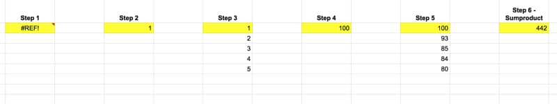
Each of these intermediary formulas in the above image moves us forward incrementally, until the final answer is obtained in step 6.

Similarly, if you’re trying to understand complex formulas, peel the layers back until you reach the core (which is hopefully a function you understand!). Then, build it back up in steps to get back to the full formula.

Example 1: Building Complex Formulas With The Onion Method

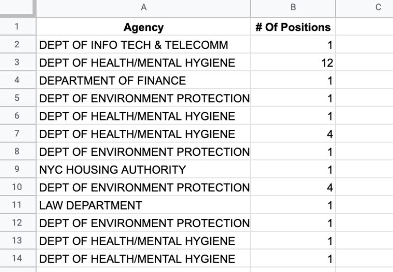
Let’s start with this job positions dataset and use the QUERY function to summarize the results:

Job position dataset

Step 1

Setup the first, simple QUERY formula to select columns A and B:

=QUERY(A1:B,"select A, B")

This doesn’t change the data, but it’s always a good idea to set up a basic query first to ensure you have the correct dataset selected as the input to your QUERY function.

Step 2

Summarize the data by job position, using a GROUP BY clause in the QUERY function:

=QUERY(A1:B,"select A, sum(B) group by A")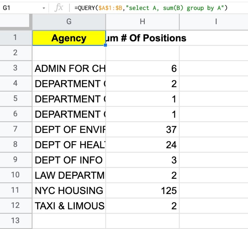

Onion Method for complex formulas

Step 3

Filter out the blank rows using the WHERE clause: “is not null”, as follows:

=QUERY(A1:B,"select A, sum(B) where A is not null group by A")

Step 4

Use an ORDER BY clause to sort the table by total in descending order:

=QUERY(A1:B,"select A, sum(B) where A is not null group by A order by sum(B) desc")

Step 5

Fix the header of the total column using the LABEL clause:

=QUERY(A1:B,"select A, sum(B) where A is not null group by A order by sum(B) desc label sum(B) 'Total Positions'")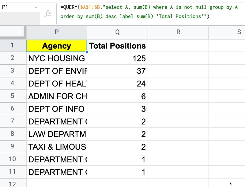

Onion Method for complex formulas

Good work!

We’ve created a pivot table using the QUERY function rather than an actual pivot table. Building it in steps, where the formula evolves slightly with each step, was key to making this work.

Let’s continue, and see how to add a total row to this QUERY formula.

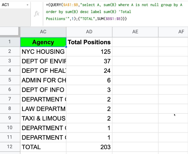
Step 6

Using array literals, add a placeholder line for the total row:

={QUERY(A1:B,"select A, sum(B) where A is not null group by A order by sum(B) desc label sum(B) 'Total Positions'");{"TOTAL","TBC"}}

Step 7

Our final step is to convert this placeholder to an actual formula, to give the correct total. As with the data input to the query function, we leave the range reference open-ended to ensure it remains dynamic and will include new data automatically:

={QUERY(A1:B,"select A, sum(B) where A is not null group by A order by sum(B) desc label sum(B) 'Total Positions'");{"TOTAL",SUM(B1:B)}}

The result is:

Onion Method for complex formulas

Example 2: Deconstructing Complex Formulas With The Onion Method

If you’re trying to understand complex formulas in Google Sheets that someone else has shared with you, you can still approach it with this Onion Method.

Simply peel back the layers until you reach the innermost function. Copy that into a new cell and start from the inside and work out, building up to the full formula again.

Let’s see an example.

Suppose we’re given this worksheet with US State names:

dataset of US State Names

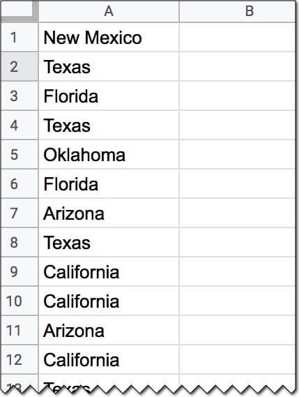
And we’re also given this formula:

=ArrayFormula(INDEX(A1:A20,MODE(MATCH(A1:A20,A1:A20,0))))

which gives an output of Texas.

But how does this formula work?

Applying The Onion Method, we peel back the layers to the core function and then build it up in steps again.