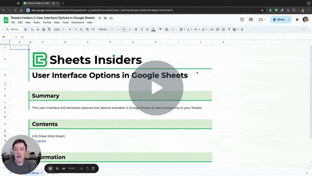
Welcome to issue 3 of the Sheets Insiders membership program.
You can see the full archives here.
You know what’s better than a great spreadsheet?
A great spreadsheet with a button!
A user interface (UI) is the way people interact with software. Here I’m using it to refer to the interactive elements we can add to our spreadsheets.
User Interface Options Template
This template presents various ways for users to interact with a Google Sheet.
You’re probably familiar with many of the techniques, but there are a surprising number of ways to add interactive elements with some creativity.
Download the User Interface Options Template
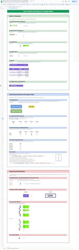
The template is divided into three sections:
- Built-in methods, which will cover 99% of use cases
- Apps Script methods, for specialized use cases
- Experimental methods, which explore the creative limits of formulas and formatting
Let’s take a closer look at each:
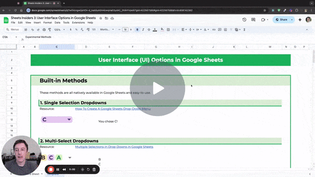
1. Built-in Methods
Explore the following built-in interactive elements in the template:
- Single dropdown
- Multi-select dropdowns
- Checkboxes
- Rating Stars
- Slicers
- Hidden rows with Group & Subtotal
You’ll find additional resources listed with each example in the template.
See also the list of ideas of how to use these features at the bottom of this post.
2. Advanced Methods with Apps Script
New to Apps Script? Start here.
Image Button
The “button” is in fact a drawing created in the Sheet.
Go to menu Insert > Drawing and create a button with the rectangle shape.
Back in your Sheet, right click on the Drawing object and then click on the 3 dots to open the menu:

Click on “Assign script” and enter the name of a function in your Apps Scrip:
clearFormatButton
Go to Extensions > Apps Script to see the scripts.
When we click on this image in the future, it will execute the “clearFormatButton” function in our script, which clears the test cell format:
function clearFormatButton() {
  const sheet = SpreadsheetApp.getActiveSheet();
  sheet.getRange('F77').clearFormat();
}
Two things to mention:
- To move the button image after you’ve assigned a script, right click it first and then you can move it.
- The first time you click the button, you’ll be prompted to grant access to the script to connect to your Google Sheet. Follow the prompts to the end and then click the button again to run the script. You only have to do this once at the beginning.
Radio Buttons with Apps Script
The radio buttons work in the template using the onEdit(e) simple trigger.
Every time the Sheet is modified (for example, when you check a checkbox), the script is called and it will check to see if the clicked cell is inside the radio box range. If it is, then it will implement the radio box controls to ensure only one checkbox is allowed within the range.
To use in your own projects, copy the code below the three lines of stars (they look like this /********/) and paste into your own script file in your Sheet.
(Access scripts in any Sheet via Extensions > Apps Script)
Change this line:
const RADIOBUTTONRANGES = ['C90:G90', 'D98:G98', 'D99:G99', 'D106:D110'];
to match the ranges of your radio button checkboxes.
For example, if you had checkboxes in A2:A8 that you wanted to act as radio buttons, modify the code to be:
const RADIOBUTTONRANGES = ['A2:A8'];
Important note:
- Ensure the ranges are wrapped with quotes (single or double quotes, just be consistent)
- Separate multiple ranges with commas
- Ensure that there is a square bracket and a semicolon ]; at the end of the line
3. Experimental Methods

Buttons with Formulas Technique
Let’s see how to build the button (#11) and sliders (#12 and #13) in the Experimental section of the template.
I’ve labeled them “Experimental” because they are finicky to set up and not particularly robust.
I wouldn’t recommend them in professional use cases, but nevertheless, it’s an interesting technique. And perhaps you’ll feel comfortable using them once you understand the limitations.
Steps
- Start with a blank Google Sheet
- Add a checkbox to cell C3
- Set the size of the checkbox to 200
- Resize the row to a normal height
- Change the font color for the cell with the checkbox to a custom color:
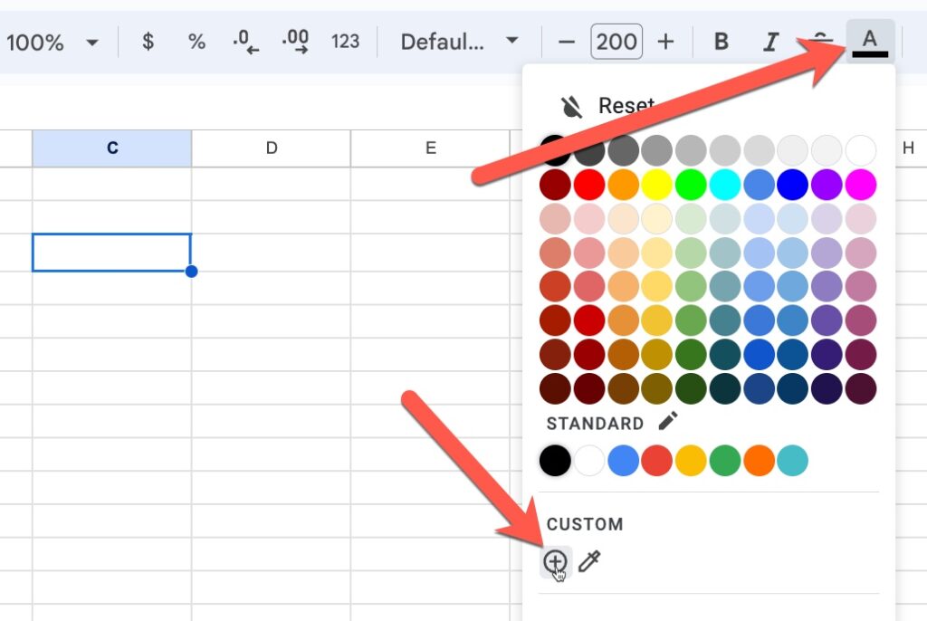
and then enter the value fffffe
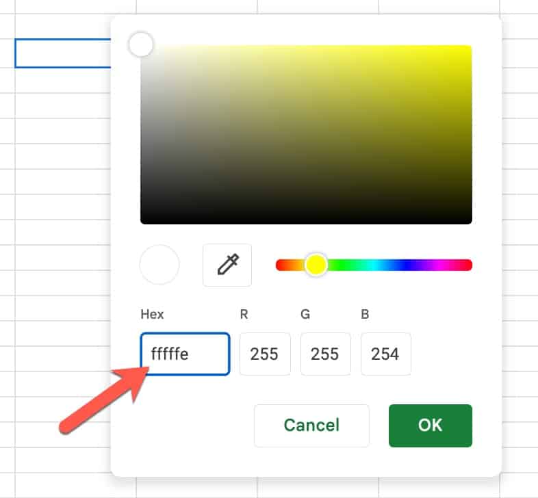
(This is one setting off pure white, so that the font and background are different to the computer but look the same to the user.)
- Click OK
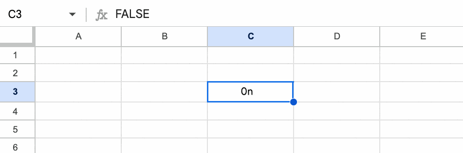
Now we have a checkbox across the entire cell C3 that is also hidden from view.
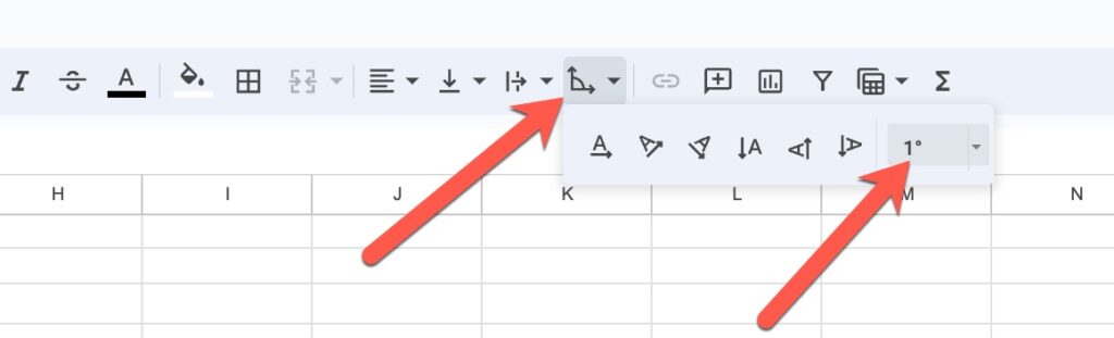
- In cell B3, enter the following formula:
=IF(C3,REPT(" ",19)&"Off",REPT(" ",19)&"On")
- In the toolbar, set the “Text rotation” to a custom value 1°
And now we have a working button where you can toggle On/Off:
How does this work?
Well, we made the checkbox bigger than cell C3 so that when we click anywhere inside the cell it triggers the checkbox.
Then we “hid” the checkbox by making the font color white. (We made it one setting different to background pure white, to avoid getting an error message that the “checkbox is not visible”.)
Then we created an IF formula to show “On” or “Off” based on the condition of the checkbox. I’m using “On” as a invitation to switch on, rather than saying it’s On already.
Finally, we use the text rotation trick to overlay this text on top of the checkbox cell. The REPT function positions the text over the checkbox cell. Feel free to adjust the value “19” in the formula to move it left or right.
This is the same technique in the sliders.
Examples using User Interface elements
- Add slicers to dashboards to let users explore different aspects of the data
- Control charts with drop-down menus (or with checkboxes)
- Build checklists with checkboxes
- Add a button to clear an invoice
- Use a checkbox to highlight data with conditional formatting
- Show/hide test hints in your Sheet with checkboxes
- Use a checkbox as a control switch for slow Sheets with big calculations