Delete Empty Rows and Columns
This is a great suggestion because it keeps your Sheets neat and tidy AND improves performance with big Sheets.
Highlight any unused rows and/or columns. Go to the menu Edit > Delete and remove them. Or use the right-click menu.
Thanks Yannis for this simple but effective tip!
Data Validation
Data validation is a technique used to check data inputs and ensure they are accurate, complete, or meet specific requirements.
Data Validation helps you catch errors long before they propagate downstream through your Sheets formulas. It helps improve the quality of your output.
Try these three methods:
- Add data validation rules under the menu: Data > Data validation.
- Use Tables, which will highlight inconsistent data entries in a column.
- Use Conditional Formatting (such as last week’s tip to highlight incomplete rows – tip #3) to bring data validation issues to the user’s attention.
Thanks to reader Ronald for sharing how he uses data validation.
He uses hidden columns to check data validation (for example, identify a blank cell that should have data). And then he uses a monitoring sheet to pull in all the errors from individual sheets, allowing him to see outstanding issues in a single place. Finally, automated email notifications, triggered via Apps Script, prompt users to fix errors directly.
Automatic Table of Contents Sheet
Adding an information sheet, with a table of contents, to the front of your important or complex sheets is a smart idea. It makes them look more professional as well as making them easier to navigate.
It’s like the difference between buying a new product in its shiny film-wrapped box versus buying the product alone. The former elicits excitement and newness. It’s similar with Sheets that have a welcoming front info sheet.
Thanks Ritesh for sharing this idea!
In fact, I advocate so strongly for including an info sheet (especially on client facing sheets) that I built my own internal add-on to generate them automatically for me. See Sheets Insiders issue 15 and issue 16 for how to do this.
Named Functions
Named Functions are super useful when you have a complex formula that you reuse over and over.
For example, reader Jes shared a named function called XQUERY. It’s a QUERY formula that works with column names from your data range, instead of standard A, B, C or Col1, Col2, Col3 notation.
It works like this:
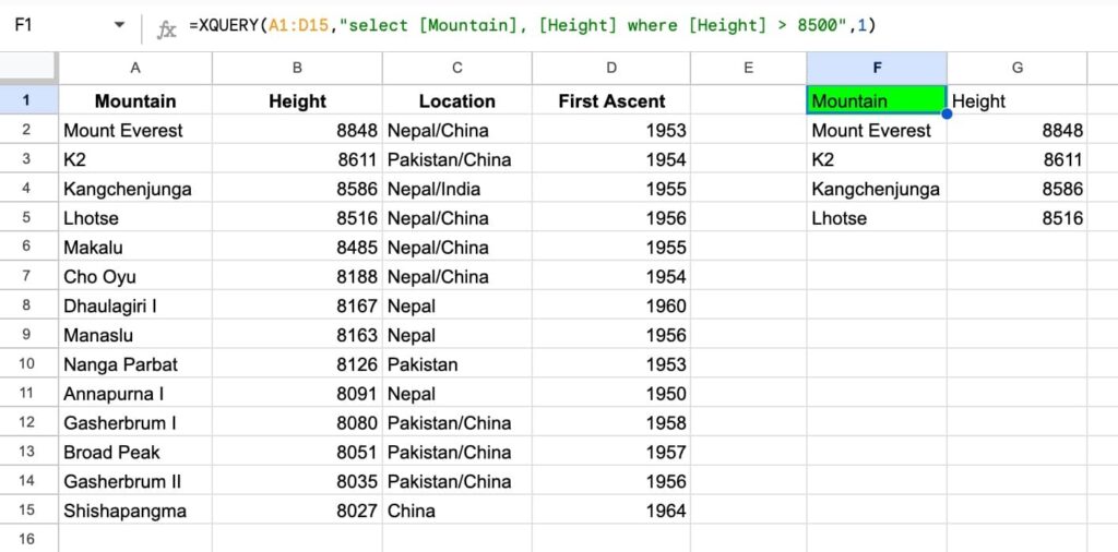
Under the hood, the named function is quite complex:
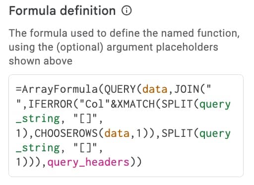
It uses XMATCH to match the header name to the column number and converts column names into Col1, Col2 type format.
Fantastic example! Thanks Jes.
Thanks also to Valère for also suggesting a named function, in this case to unpivot wide tables with an unlimited number of columns & headers. Another great example!
Build Strings With Formulas
If you’re a developer, then this is a real time saver.
You can use formulas to build strings to use in other coding platforms.
For example, Jose shared how he uses this formula to convert lists in Sheets into text strings that can be used inside SQL queries.
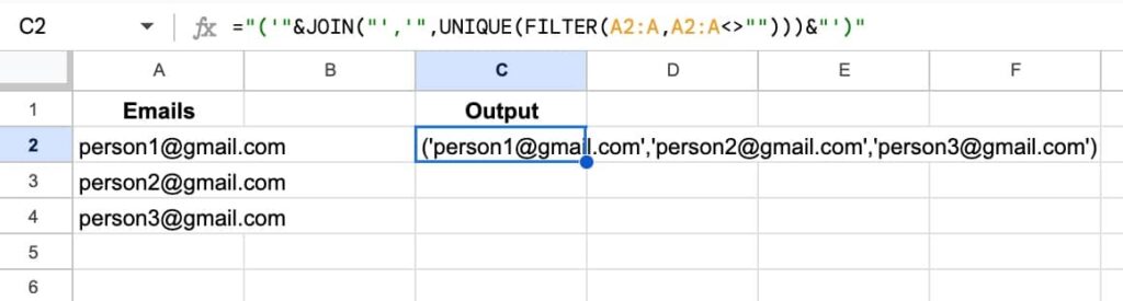
The formula is:
="('"&JOIN("','",UNIQUE(FILTER(A2:A,A2:A<>"")))&"')"
It turns the list of email addresses in column A into a comma-separated list with single quotes, inside brackets.
This output can then easily be copy-pasted into SQL queries:
select * from clients where email IN (‘person1@gmail.com’,’person2@gmail.com’,’person3@gmail.com’)
Thanks, Jose!
I’ve used this technique myself many times over the years to turn Google Sheet content into HTML/CSS content for my website.
For example, this formula converts data from cells A1 and A2 into an HTML header:
="<h1>"&PROPER(A1)&"</h1>"&REPT(CHAR(10),2)&"<div class=""codewrapper""><code>"&A2&"</code></div>"
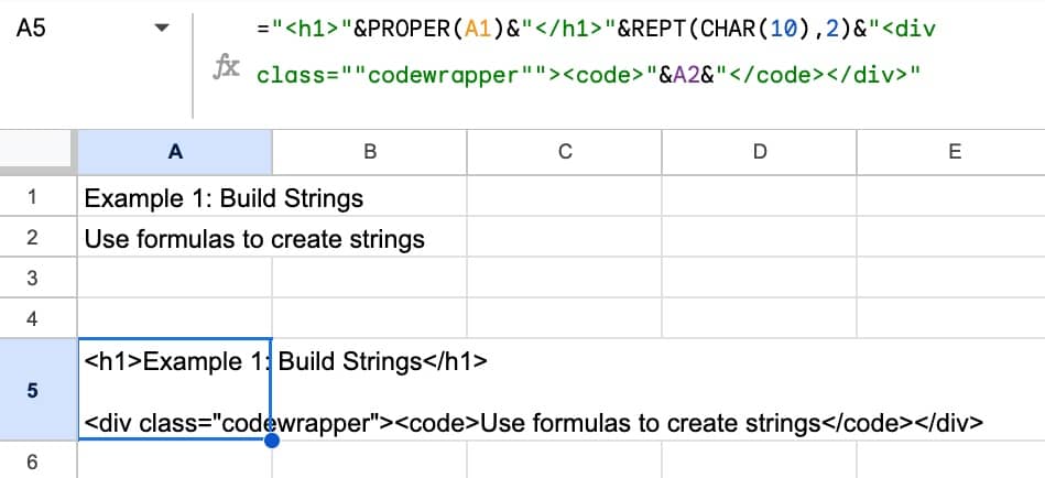
I can now copy-paste this text directly into my HTML file.
Highlight All Formula Cells with Conditional Formatting
In last week’s email, we saw how to use conditional formatting to apply a global comment system. This tip is very similar.
Highlight your entire Sheet by clicking that little box at the top left, between the “A” and the “1”.
Then go to the menu Format > Conditional Formatting
Add this custom formula rule:
=ISFORMULA(A1)
Change the format to highlight the cell by, for example, changing the font color or background color.
Now, anytime you use a formula in a cell, it will highlight it in a special way.
Thanks Dan for this idea!