18 Best Practices for Working with Data in Google Sheets

This article outlines 18 best practices for working with data in Google Sheets.

It’s a compilation of my own experiences of working with data in spreadsheets for 15+ years, along with the opinions of others I’ve worked with and reports and articles I’ve read online.

By no means is it meant to be exhaustive or the last word on the subject, but if you follow these guidelines, you should have a robust data workflow.

Following these best practices for working with data will make you more efficient and reduce the chance of errors creeping in. It’ll make your work easier to follow and understand and add value to your team’s or client’s workflow process. It’s a good habit to have, and it’ll serve you well as you progress with your data career.

Contents

1. Organize your data
2. Keep a backup copy of your data
3. Document the steps you take
4. Go with wide-format data tables
5. Use good, consistent names
6. Use data validation for data entry
7. Even better, use Google Forms for data entry
8. One cell = one piece of information
9. Distinguish columns you add
10. Don’t use formatting to convey data
11. Add an index column for sorting & referencing
12. Format the header row
13. Freeze the header row
14. Turn formulas into static values after use
15. Keep copies of your formulas
16. Create named ranges for your datasets
17. Avoid merged cells
18. Tell the story of one row

18 best practices for working with data

1. Organize your data

Projects are more likely to be successful when there is good communication and a good organizational structure. A big piece of that is good data management, and that starts with implementing a well-organized, logical and efficient folder structure.

As your projects grow in size, it becomes more and more crucial to keep your Google Sheets organized in a meaningful way.

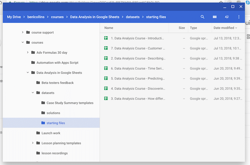
At a minimum, you’ll have a top level project folder and inside that, you’ll want separate folders for your raw datasets, for your analysis and for your final deliverables. Files can move from one folder to the next (or be copied from one folder to the next) as the project progresses.

Here’s an example from my Drive, with folders for each course I’m working on, and sub-folders within them:

2. Keep a backup copy of your data

Surely this is redundant in the age of cloud data, right?

On the one hand yes, there shouldn’t be a need to backup your Google Sheets.

Google has so much redundancy built in, your data should be safe from getting corrupted or lost. And you can rely on version history to go back in time to an earlier version of your Sheet should you need to. You can restore files from trash, although once you’ve deleted them from trash they really are gone for good (I believe there’s an exception for admins of school G Suite accounts however).

So your data should be safe.

On the other hand, however, your account could still get hacked or a colleague could (accidentally) delete a crucial file, and you could lose data that way.

For anything that’s really important, it’s worth making a copy, either in a different google account if you have one, and/or offline (as a CSV or excel file).

It’s definitely not necessary for everything, just your mission-critical stuff.

It’s also worth mentioning that making a copy of a Sheet means the new copy does not have the version history, which can be an advantage or disadvantage depending on your situation. It’s generally a good idea if you’re sharing the Sheet and don’t want anyone to be able to see all your workings to get to the final result (maybe you deleted confidential data for example).

3. Document the steps you take

This is often left as an afterthought or worse, just not done at all. However, it’s absolutely one of the best practices for working with data. It just requires a little effort.

There’ll come a day when you’re glad of some notes about where your data came from, what assumptions you made, what calculations you decided to do, and how you did them!

It doesn’t need to be super long, just enough detail to allow you or someone else enough information to understand and recreate the analysis.

This is example is deliberately detailed, so I wouldn’t suggest you need to create something like this everytime:

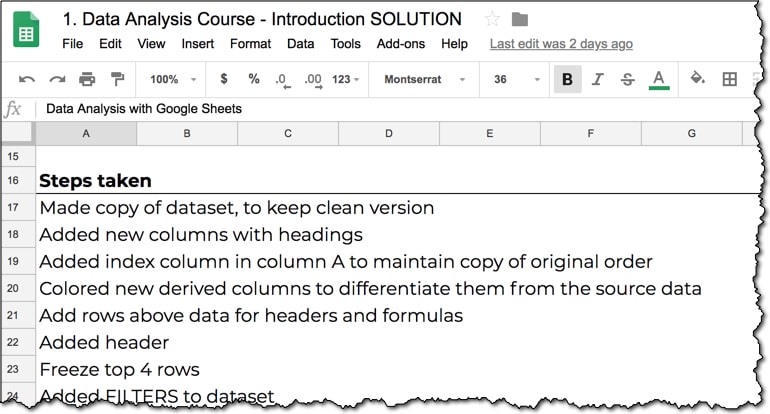
However, it would be worth mentioning where your data came from, what major steps or tests you did, and how you did them (e.g. “Ran pivot table to determine aggregate sales metrics”), as well as any assumptions you made.

If you’re creating a dataset, then you should also create a data dictionary, where you explain what data each column holds. A data dictionary is just a list of column headings in a separate tab, with a note explaining each column, for example, what the units are, whether it’s been normalized, how it’s been calculated etc.

4. Understand wide-format and tall-format data tables

As spreadsheet users, we typically use 2-dimensional, wide-format tables.

The rows and columns represent categories or measures (for example, regions vs. months). It’s easy to understand this grid format and charts and calculations lend themselves better to this layout since you can run calculations across rows or columns.

The Google Sheets chart tool expects data in a “wide-format” table rather than a traditional “tall-format” table (which is how data is stored in databases).

This “wide-table” format makes it easy for the chart tool to parse the data and show it correctly.

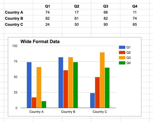
There are no blank rows or columns. The X values (the Countries) are in the first column and the series names (the Quarters) are in the first row.

Contrast that with a “tall-table” format (how a database typically stores data) and you can see the chart tool cannot correctly parse and show the data.

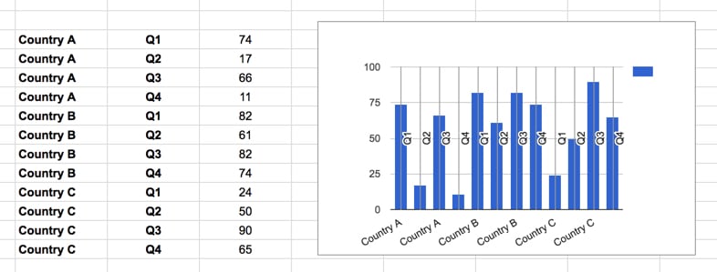
However, the tall-format datasets work much better for doing data analysis, with Pivot Tables or the QUERY function.

To transform tall data into wide data is called a pivot.

To transform wide data into tall data is a harder operation and is called unpivot. Here’s how to use the FLATTEN function and the SPLIT function to unpivot in Google Sheets.

Note: this is not a case of right and wrong, and you’ll encounter data in both formats and even in between. It’s about using the right shape for the context of your situation.

Do you want to create a chart from your data table? Go wide! Do you want to export your data table as a CSV for uploading to your company database? Maybe you’ll need to create a tall format table then.

For further reading on this subject, check out this excellent post, Spreadsheet Thinking vs Database Thinking, from Robert Kosara.

5. Use good, consistent names

As your projects grow in size and complexity it pays to develop a consistent naming strategy for your Sheets, for tabs, named ranges, variables, and column headings.

Historically, computer programmers have avoided spaces in variable names, and although it’s not strictly necessary in Sheets, it’s still a good idea to avoid spaces and non-alphanumeric characters in tab names, named ranges and column names.

Why?

Certain functions (e.g. inside the select statement of the QUERY function) and certain add-ons still adhere to this strict no-space rule, so although not very common, it will save you hassle.

The preferred approach is to use camel case or underscore notation, and you can choose whichever you prefer, e.g.:

customerData

customer_data

6. Use data validation for data entry

One of the most time-consuming tasks data practitioners face is tidying up and cleaning data.

The problem is more acute wherever there is user-generated content. Invariably, everyone will use different notations (e.g. US, USA, United States, America, US of A,…), or misspell names, or enter dates with month first vs. day first, etc.

Anything you can do to preempt this will save you lots of time on the back-end when you’re working with the data.

One method is to use Data Validation to control what a user can enter into a cell. For example, you could present them with a drop-down list of choices (instead of a free-form field), or restrict the cell to numbers only, or to positive numbers only, or all sorts of other data validation options.

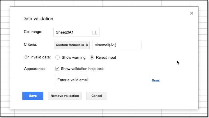
Here’s a more detailed example, combining the ISEMAIL function with data validation to ensure only valid email addresses can be entered into your Sheets, ensuring better data accuracy going forward.

In the cell where an email address will be entered, for example A1 in the image above, right click and choose Data Validation... or go to Data > Data Validation... menu option, which opens this popup.

Choose Custom Formula in the second option and enter =ISEMAIL(A1), as shown in this image:

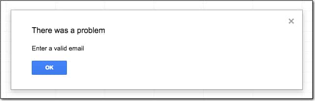
This prevents a user from entering an invalid email, or anything other than an email, into that cell, and displays a warning sign and leaves the cell empty:

7. Even better, use Google Forms for data entry

Google Forms are an even more robust way to collect user inputs because it separates the data collection from the data storage/analysis. This will prevent users from accidentally (or intentionally) overwriting data and/or seeing data from other users.

They’re super easy to set up and pair seamlessly with Google Sheets. I use them for all of my own audience surveys and course feedback surveys.

I’ve written about using Google Forms before, in this article.

8. One cell = one piece of information

Each cell should contain just one piece of information. Don’t be tempted to put more than one datapoint into a cell.

Cells with single data points can be used in formulas and charts without issues. Those with multiple data points, well, they can’t.

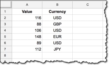
For example, if your dataset has different currency values, then you’ll want to use two columns to record the data, one for the value, and one for the currency, like this:

This is much better than having a column like this in your dataset:

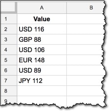
Note, you often get data in this format, with multiple data points encoded in a single cell, and it’s your job to split that data out into separate columns, so you can do your analysis.

9. Distinguish columns you add (e.g. by color)

It’s helpful to be able to distinguish the original raw data from any columns you’ve added in the course of your analysis. You’ll quickly lose track of the original data columns if you don’t mark them, and I’ve found adding a subtle color to the whole column is the quickest and most reliable way of indicating this.

Can you tell which are the original and which are the columns I’ve added in this example?

10. Don’t use formatting to convey data

Another color tip amongst the best practices for working with data in Google Sheets!

Don’t use formatting exclusively to communicate data, merely to augment underlying data.

Having just told you in the previous tip to distinguish columns by color, I’m now telling you not to? What?!?

This is different.

In the previous point, color was used to make your life simpler, to help you quickly identify what was original data and what was calculated columns you’ve added. It’s not communicating data, it’s simply facilitating a more efficient workflow.

In this case, suppose you want to classify revenue numbers into ones that require follow up versus ones that don’t. If you use cell highlighting to identify the ones you want to follow up with, you risk that not being understood by other users or worse, being lost if you export your Sheet to CSV, or someone decides to make wholesale changes to the formatting.

You want to avoid the situation on the left, and instead follow the example on the right, where data is communicated explicitly:

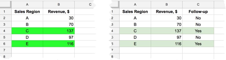
The color is merely a tool to aid comprehension, to make it easier and quicker for the user to work with your data.

11. Add an index column for sorting & referencing

Anytime you find yourself sorting your data, for example to rank largest to smallest for metric X, then you’ll want to add an index column, which will allow you to always get back to the original order.

It’s a simple numeric counter on each row, starting from 1 and going up to the last row of your dataset:

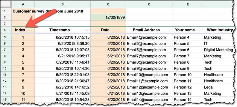
You’ll notice that it’s a colored column, meaning it’s one that I’ve added to the dataset.

I’ve been stuck before, unable to reverse the numerous sorts I’d performed and left with a dataset in an order than no longer made sense. There’s a number of reasons why you might want to get back to the order the data came in, perhaps to check for the sequence transactions happened in, perhaps to explain your steps to somebody else, or for sharing the data with other users.

12. Format the header row best practices for working with data

Center your column headings.

Wrap header text.

Make header text bold.

That’s all!

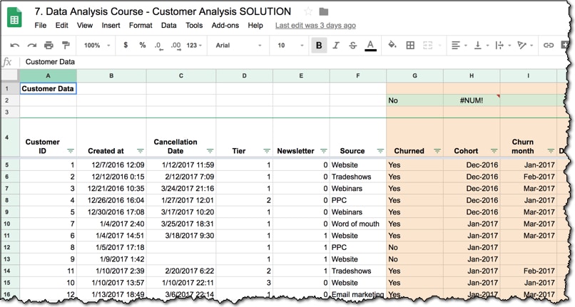
13. Freeze the header row

Hopefully this is already one of the best practices for working with data that you follow.

This should be something you do automatically without thinking. It’s essential once you have more than 20 rows of data, otherwise you’ll lose track of your column headings.

Find this in the View menu: View > Freeze > Up to current row

This is how locked top rows behave when you scroll:

14. Turn formulas into static values after use

Once you’ve used a formula, it’s generally a good idea to turn those “live” formulas into static values, provided you don’t need to keep them active.

There are times when you need to keep your formula active because your data is changing and you want the formulas to update in real-time. In that case, it’s totally fine to leave “live” formulas in your dataset.

However, if you’ve used a formula to derive a column, for example an IF based on a static date column, and it’s not going to ever change again, then you should change the column into static values.

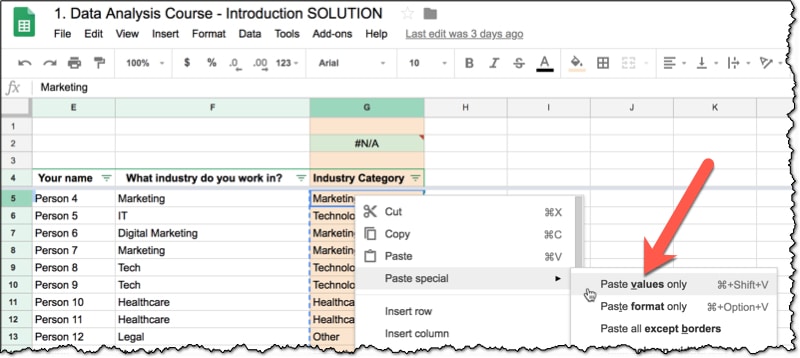
Highlight the whole column and copy the data (Cmd + C on a Mac, or Ctrl + C on a PC/Chromebook).

Then over the top of this same data range, Paste-Special-As-Values.

Either right click and select Paste special > Paste values only or use the shortcut: Cmd + Shift + V on a Mac, or Ctrl + Shift + V on a PC/Chromebook.

This will help to make your Sheets run quicker, which is an important factor if you have large amounts of data.

15. Keep copies of your formulas

In the previous step, I advocated turning formulas that you’ve used into static values, once you’re finished with them.

However, you should definitely keep a copy of them!

You’ll thank yourself later when you need to re-use it, and you have it available, or when someone asks you how you derived a certain column.

By far the most convenient way to keep a copy of formulas is to paste a live copy into a row above your dataset and leave it there. That way it’ll keep all the relative references intact, so you can quickly copy it into your dataset to use again.

Here’s an example and you’ll notice that I’ve colored the formula green, to indicate I have a live formula in that cell:

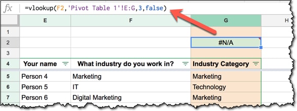
Don’t worry if the formula shows an #N/A!, a blank cell or even a wrong answer, what matters is that it keeps the relative references intact.

You can simply copy the formula from your column into the row above, and vice-versa, and know that it’ll just work:

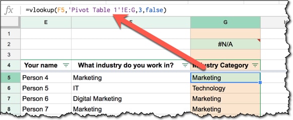
Once you’ve copied your formula into the row above your dataset, feel free to copy-paste-special-values and turn the column into static values as per the previous best practice.

Important Note: Purists will argue that you should have a single header row and nothing more. I think there are pros and cons to this header-row-only approach and the “utility” row approach I’ve advocated here.

I use both methods, but tend to favor the approach of having a few “utility” rows because I think the benefits of keeping copies of formulas above your data analysis workings is worth the small price to pay to not start in row one. And once you’ve setup your named ranges, the issue falls away anyway.

One scenario that I would definitely go with a single header row approach is if I was creating a flat dataset (no formulas) to be shared.

16. Create named ranges for your datasets

This is a good habit to get into, and saves you having to manually highlight your data or type in the range reference every time you refer to your data in a formula.

It’ll reduce errors from incorrect range references or mixing up relative/absolute references, and has the added benefit of making your formulas clearer to understand.

Find it in the Data menu: Data > Named ranges...

It’s the difference between this, clean simple syntax:

and this, where you have to highlight the range you want:

17. Avoid merged cells

One of the most important of the best practices for working with data in Google Sheets.

Merged cells should be avoided in datasets.

They cause all sorts of problems in datasets: they break formulas, nobody will know which column or row they relate to, your data gets overwritten, etc…

I’m not suggesting you never use merged cells (here’s how to use merged cells in Google Sheets correctly), because they can be useful.

For example, they let you position elements when you’re building front-end applications for Google Sheets and you want to get a certain layout, as shown in the header of this Facebook dashboard:

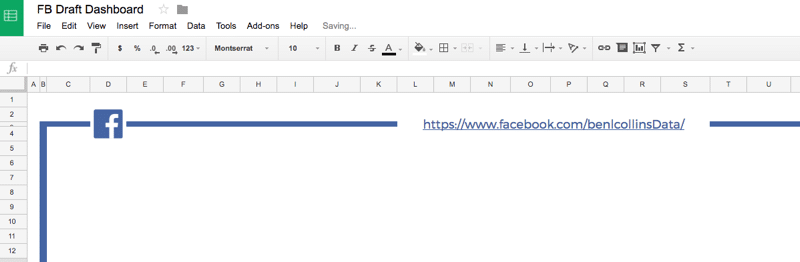
Just not in your datasets, ok!

18. Tell the story of one row

This is perhaps my favorite of the 18 best practices for working with data, because it’s so simple but so effective.

This is a useful tip I picked up from a data scientist at General Assembly in Washington, DC, when I was teaching their Data Analysis course in 2015/16.

The idea is to read (out loud if you like!) across one row of your data and really see and understand what’s in every column.

It’ll help you know what data is in your dataset, or prompt you to investigate further if you don’t understand what a column shows. Potentially it’ll save you doing unnecessary work, because you’ll know exactly what you have.

Developers often keep yellow rubber duckies sitting on their desks to debug their lines of code, so go ahead and follow their example if you like!

Further reading:

A tweet from data scientist Hadley Wickham, containing a wealth of ideas and opinions.

Data organization in spreadsheets, a research paper by Karl Broman and Kara Woo.

Best Practices for Using Google Sheets in Your Data Project by Matthew Lincoln.

Anything you’d like to add? Do you follow any best practices for working with data that are different from what I’ve described here? Drop a note in the comments!

Related Articles