The Google Sheets Query function is the most powerful and versatile function in Google Sheets.
It allows you to use data commands to manipulate your data in Google Sheets, and it’s incredibly versatile and powerful.
This single function does the job of many other functions and can replicate most of the functionality of pivot tables.
This video is lesson 14 of 30 from my free Google Sheets course: Advanced Formulas 30 Day Challenge
Google Sheets QUERY Function Syntax
=QUERY(data, query, [headers])It takes 3 arguments:
- the range of data you want to analyze
- the query you want to run, enclosed in quotations
- an optional number to say how many header rows there are in your data
Here’s an example QUERY function:
=QUERY(A1:D234,"SELECT B, D",1)The data range in this example is A1:D234
The query statement is the string inside the quotes, in green. In this case, it tells the function to select columns B and D from the data.
The third argument is the number 1, which tells the function that the original data had a single header row. This argument is optional and, if omitted, will be determined automatically by Sheets.
It’s one of the Google-only functions that are not available in other spreadsheet tools.
QUERY Function Notes
The keywords are not case sensitive, so you can write “SELECT” or “select” and both work.
However, the column letters must be uppercase: A, B, C, etc. otherwise you’ll get an error.
The keywords must appear in this order (of course, you don’t have to use them all):
- select
- where
- group by
- order by
- limit
- label
You’ll see examples of all of these keywords below.
There are a few other keywords but they are much less common. See the full list here.
 💡 Learn more
Learn more about the QUERY Function in my newest course: The QUERY Function in Google Sheets
Google Sheets QUERY Function Template
Click here to open a view-only copy >>
Feel free to make a copy: File > Make a copy…
If you can’t access the template, it might be because of your organization’s Google Workspace settings. If you right-click the link and open it in an Incognito window you’ll be able to see it.
Google Sheets QUERY Function Examples
If you want to follow along with the solutions, please make a copy of the Google Sheet template above.
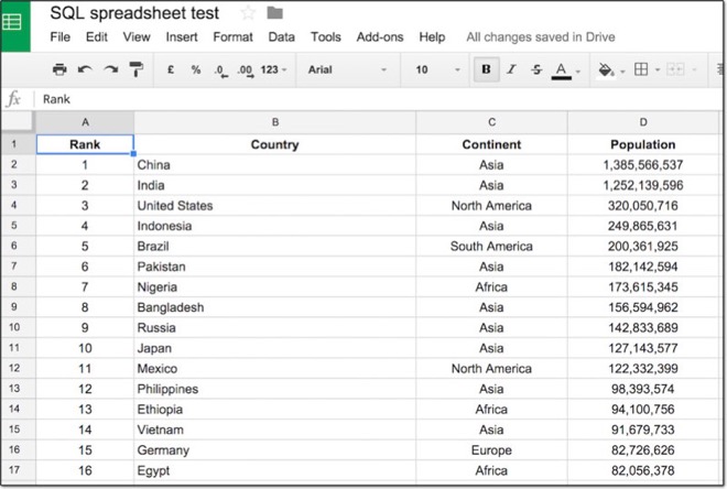
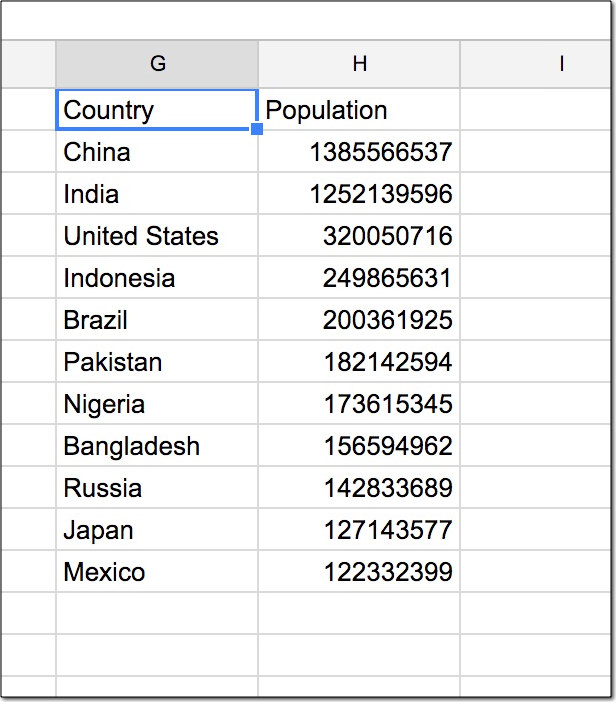
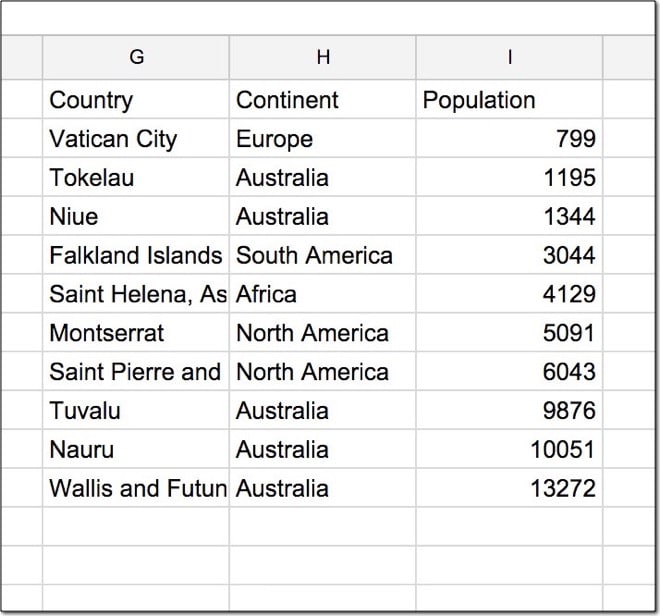
This is what our starting data looks like:
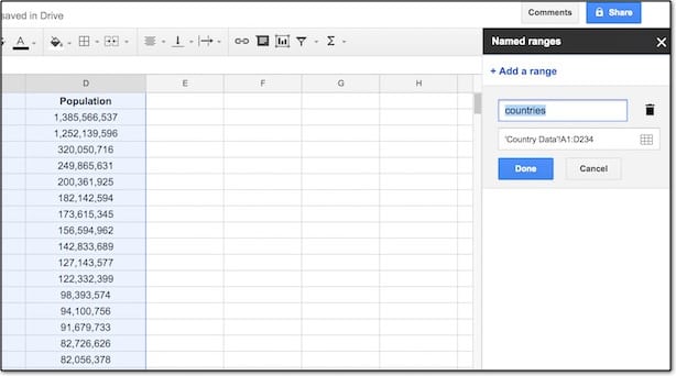
In this tutorial, I have used a named range to identify the data, which makes it much easier and cleaner to use in the QUERY function. Feel free to use the named range “countries” too, which already exists in the template.
If you’re new to named ranges, here’s how you create them:
Select your data range and go to the menu:
Data > Named ranges…
A new pane will show on the right side of your spreadsheet. In the first input box, enter a name for your table of data so you can refer to it easily.
SELECT All
The statement SELECT * retrieves all of the columns from our data table.
To the right side of the table (I’ve used cell G1) type the following Google Sheets QUERY function using the named range notation:
=QUERY(countries,"SELECT *",1)Notes: if you don’t want to use named ranges then that’s no problem. Your QUERY formula will look like this:
=QUERY(A1:D234,"SELECT *",1)For the remainder of this article, I’ve used the named range “countries” but feel free to continue using the regular range reference A1:D234 in its place.
The output from this query is our full table again, because SELECT * retrieves all of the columns from the countries table:
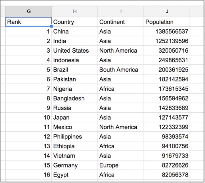
Wow, there you go! You’ve written your first QUERY! Pat yourself on the back.
SELECT Specific Columns
What if we don’t want to select every column, but only certain ones?
Modify your Google Sheets QUERY function to read:
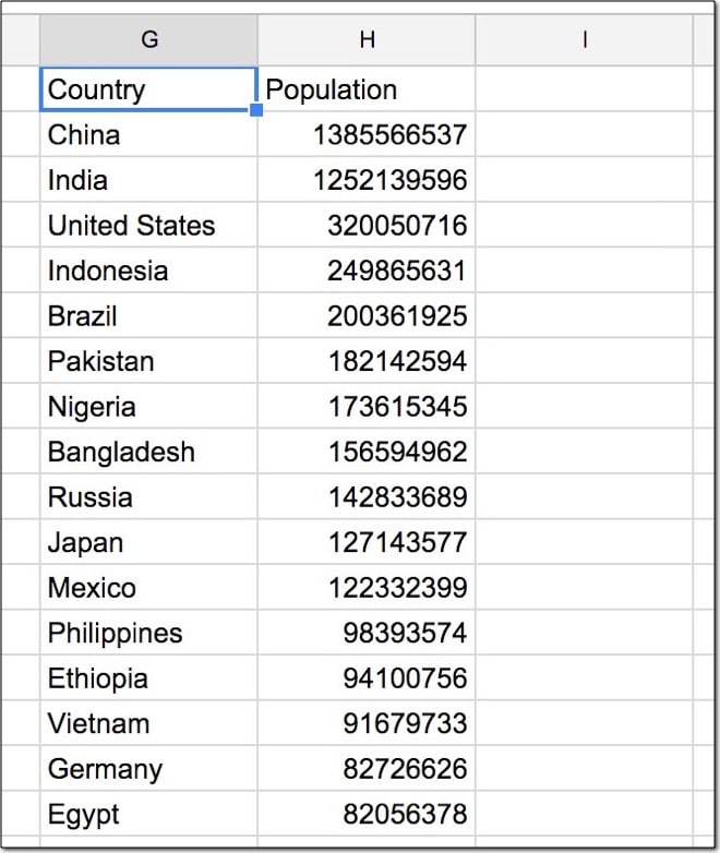
=QUERY(countries,"SELECT B, D",1)This time we’ve selected only columns B and D from the original dataset, so our output will look like this:
Important Note
Remember, our QUERY function is in cell G1, so the output will be in columns G, H, I, etc.
The B and D inside the QUERY select statement refer to the column references back in the original data.
WHERE Keyword
The WHERE keyword specifies a condition that must be satisfied. It filters our data. It comes after the SELECT keyword.
Modify your Google Sheets QUERY function to select only countries that have a population greater than 100 million:
=QUERY(countries,"SELECT B, D WHERE D > 100000000",1)Our output table is:
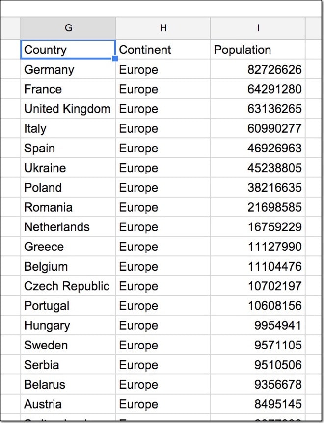
Let’s see another WHERE keyword example, this time selecting only European countries. Modify your formula to:
=QUERY(countries,"SELECT B, C, D WHERE C = 'Europe' ",1)Notice how there are single quotes around the word ‘Europe’. Contrast this to the numeric example before which did not require single quotes around the number.
Now the output table is:
ORDER BY Keyword
The ORDER BY keyword sorts our data. We can specify the column(s) and direction (ascending or descending). It comes after the SELECT and WHERE keywords.
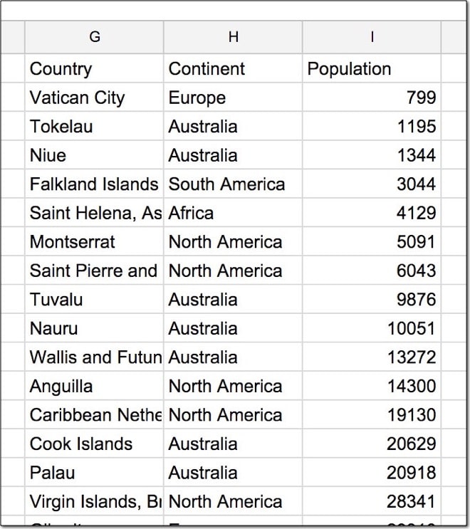
Let’s sort our data by population from smallest to largest. Modify your formula to add the following ORDER BY keyword, specifying an ascending direction with ASC:
=QUERY(countries,"SELECT B, C, D ORDER BY D ASC",1)The output table:
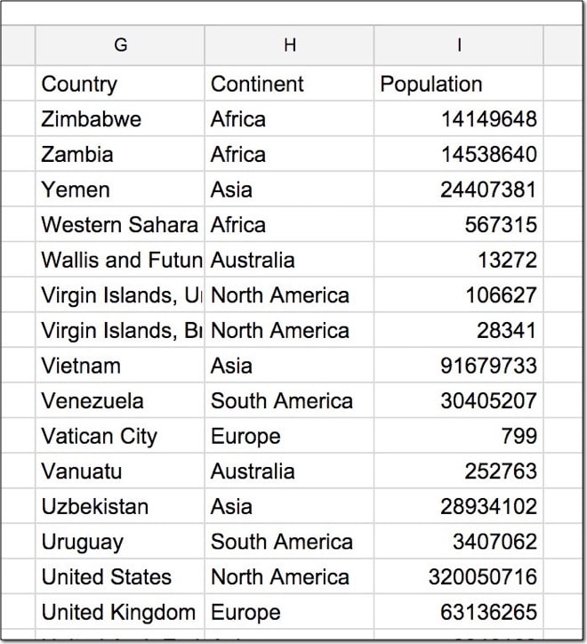
Modify your QUERY formula to sort the data by country in descending order, Z – A:
=QUERY(countries,"SELECT B, C, D ORDER BY B DESC",1)Output table:
LIMIT Keyword
The LIMIT keyword restricts the number of results returned. It comes after the SELECT, WHERE, and ORDER BY keywords.
Let’s add a LIMIT keyword to our formula and return only 10 results:
=QUERY(countries,"SELECT B, C, D ORDER BY D ASC LIMIT 10",1)This now returns only 10 results from our data:
Arithmetic Functions
We can perform standard math operations on numeric columns.
So let’s figure out what percentage of the total world population (7.16 billion) each country accounts for.
We’re going to divide the population column by the total (7,162,119,434) and multiply by 100 to calculate percentages. So, modify our formula to read:
=QUERY(countries,"SELECT B, C, (D / 7162119434) * 100",1)I’ve divided the values in column D by the total population (inside the parentheses), then multiplied by 100 to get a percentage.
The output table this time is:
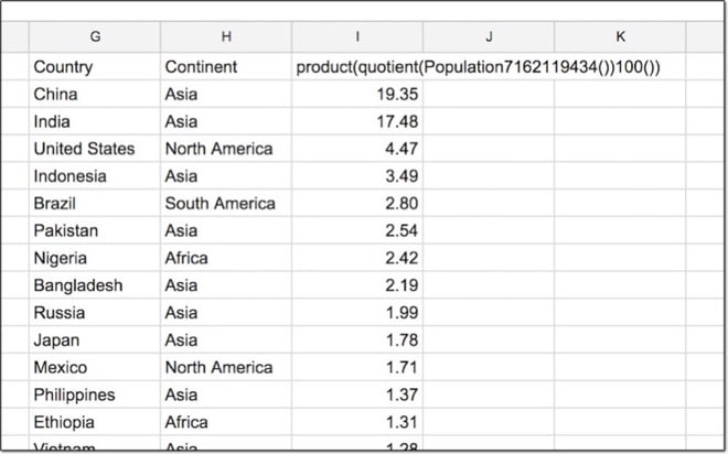
Note – I’ve applied formatting to the output column in Google Sheets to only show 2 decimal places.
LABEL Keyword
That heading for the arithmetic column is pretty ugly right? Well, we can rename it using the LABEL keyword, which comes at the end of the QUERY statement. Try this out:
=QUERY(countries,"SELECT B, C, (D / 7162119434) * 100 LABEL (D / 7162119434) * 100 'Percentage'",1)
=QUERY(countries,"SELECT B, C, (D / 7162119434) * 100 LABEL (D / 7162119434) * 100 'Percentage' ",1)Aggregation Functions
We can use other functions in our calculations, for example, min, max, and average.
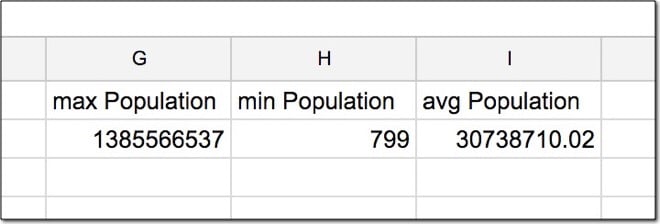
To calculate the min, max and average populations in your country dataset, use aggregate functions in your query as follows:
=QUERY(countries,"SELECT max(D), min(D), avg(D)",1)The output returns three values – the max, min and average populations of the dataset, as follows:
GROUP BY Keyword
Ok, take a deep breath. This is the most challenging concept to understand. However, if you’ve ever used pivot tables in Google Sheets (or Excel) then you should be fine with this.
The GROUP BY keyword is used with aggregate functions to summarize data into groups as a pivot table does.
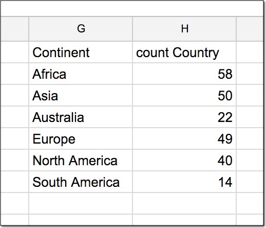
Let’s summarize by continent and count out how many countries per continent. Change your query formula to include a GROUP BY keyword and use the COUNT aggregate function to count how many countries, as follows:
=QUERY(countries,"SELECT C, count(B) GROUP BY C",1)Note, every column in the SELECT statement (i.e. before the GROUP BY) must either be aggregated (e.g. counted, min, max) or appear after the GROUP BY keyword (e.g. column C in this case).
The output for this query is:
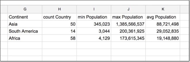
Let’s see a more complex example, incorporating many different types of keyword. Modify the formula to read:
=QUERY(countries,"SELECT C, count(B), min(D), max(D), avg(D) GROUP BY C ORDER BY avg(D) DESC LIMIT 3",1)This may be easier to read broken out onto multiple lines:
=QUERY(countries,

"SELECT C, count(B), min(D), max(D), avg(D)

GROUP BY C

ORDER BY avg(D) DESC

LIMIT 3",1)
This summarizes our data for each continent, sorts by highest to the lowest average population, and finally limits the results to just the top 3.
The output of this query is:
Advanced Google Sheets QUERY Function Techniques
How to add a total row to your Query formulas
How to use dates as filters in your Query formulas
There are 4 more keywords that haven’t been covered in this article: PIVOT, OFFSET, FORMAT and OPTIONS.
In addition, there are more data manipulation functions available than we’ve discussed above. For example, there are a range of scalar functions for working with dates.
Suppose you have a column of dates in column A of your dataset, and you want to summarize your data by year. You can roll it up by using the YEAR scalar function:
=QUERY(data,"select YEAR(A), COUNT(A) group by YEAR(A)",1)For more advanced techniques with the QUERY function, have a watch of this lesson from the Advanced 30 course:
This video is lesson 15 of 30 from my free Google Sheets course: Advanced Formulas 30 Day Challenge.
Other Resources
The QUERY Function is covered in days 14 and 15 of my free Advanced Formulas course for Google Sheets: Learn 30 Advanced Formulas in 30 Days
Official Google documentation for the QUERY() function.
Official documentation for Google’s Visualization API Query Language.
Brilliant, yet again.
Thanks!
Dear Ben,
You’re very expert and helpful as I found in this content. Would you please advice me the right query of below?
=query(FirstEntry!A2:Y, “Select * Where K ='”Dashboard!W2″‘”)
https://docs.google.com/spreadsheets/d/1DpM0m2T6xYOcg5YZru-ZP4sz6tPTti92mLEPBF9bG20/edit?usp=sharing
All red marks in Dashboard(W2) and DataBank (A3) pages. Really Thanks for your kind support. Have a nice day.
You have to insert the value of the feild, not the name. This is how to do it:
=query(FirstEntry!A2:Y, “Select * Where K ='” & Dashboard!W2 & “‘”)
Note the single quotes, one after the equal sign and another between double quotes just before the closing bracket.
This is very helpful.Thank you for the contribution
Hi ,
I did this trying to reference a text sting in a cell, so i can copy the cell function to next row but cell reference keeps the A2.
=query(Entries,”select C,H where C=’”& Horses!A2&“ ‘ “,)
take a look at “,” at the end just before “)” -it makes the error
=query(FirstEntry!A2:Y, “Select * Where K =’”&Dashboard!W&″‘ ”)
Hi
Is there a way to extract all columns except col3,col5. i have around 200 columns but i want to exclude few columns from those 200 columns
Hi Ramesh,
You can use other formulas to build the list of column IDs inside the QUERY function, to save having to type them out. For example, this formula selects column 1 and 2, and then uses a reduce function to select columns 5 to 105:
=QUERY({A:P},"select Col1, Col2"&REDUCE("",SEQUENCE(100,1,5,1),LAMBDA(a,c,A&", Col"&c)))You can change the value “100” to however many columns you have, and the value “5” for the start column number.
Hope this helps!
Ben
Ben thanks a lot! With the new tables in google sheets, you cannot do select A, B, C.
Instead you have to use Col1, Col2 and luckily I stumbled upon your comments because I could not find the correct syntax. Do you know how to concatenate two text columns together?
i need From Bigquery and metabase Queried results must be displayed on Google sheets and has to be automated using R
I have a livestock feed shopping worksheet to show a range of start and end dates with specific initial vendors. to display the date range I have managed to create a query function, but at the same time only sort by vendor-specific. What function should I use to accompany the query function?
Is it possible to use column titles instead of the letters in the query? As in, SELECT MAX(Population)
Hi Alex – no, unfortunately you can’t use the column titles inside the QUERY function in Google sheets (see this Stack Overflow thread for some discussion on this subject). The only other variation I’ve seen is the ability to use “Col1”, “Col2”, “Col3” etc. when you combine the QUERY function with one of the IMPORT functions, e.g. try this:
=query(importhtml("https://en.wikipedia.org/wiki/The_Simpsons","table",3),"select Col1, Col4, Col8 where Col8 > 25",1)For details on this, check out this introduction on Stack Overflow.
Thank you, Ben!
`importhtml` is another useful function I didn’t know about
Hey Alex, you might also enjoy this post then: https://www.benlcollins.com/spreadsheets/import-social-media-data/
All about ImportXML and ImportHTML functions.
Cheers, Ben
Hi Ben and Alex,
I had the same question and I think there is a solution for it, you just need to combine the query() function with substitute & match:
=query(A17:E20, "Select "&SUBSTITUTE(ADDRESS(1,MATCH("Status",$17:$17,0),4),"1","")&" ")Basically this is combining query() with the SUBSTITUTE() function to turn a column number into a letter, and then we’re using MATCH() to look for the column number with the header name we need (in my example ‘Status’), in the range of the headers (my example $17:$17). And that’s it!
Nice solution Johannes! Thanks for sharing here!
Cheers,
Ben
Hi Ben,
I’m taking your 30 Day Advanced Formula challenge – it’s been fun! And it inspired me to see if I could use the column() formula to insert the Col# for me when using Queries with ImportRange.
I gave it a try, and it was a success! Here’s a short example:
=QUERY(IMPORTRANGE(“…”,”Data!A:Z”),”Select
Col”&Column(B:B)&
“, Col”&Column(X:X)&
” WHERE Col”&Column(X:X)&”= ‘Chicago'”
,1)
This method looks a little cleaner than substitute & match, but you have to do know which column you want to refer to. What are your thoughts?
Thanks for all the great content!
I’d like to add that you can also use “Col1”, “Col2”, “Col3” etc: whenever the “data” argument of the QUERY() is an array. So, you could do something like this:
=QUERY({A1:Z}, “select Col1, Col4, Col8 where Col8 > 25”, 1)
Thank you very much for taking the time to create such quality content!!
This was really useful, thank you.
I’m struggling to use arithmetic operators in a query. I want to minus the sum of one column from the sum of another. My instinct says
query(data, “select D, (Sum(E) – Sum(G)) group by D where E>G”,1) but that doesn’t work :/
Any guidance would be gratefully received!
Hey Jonathan,
You were really close but the WHERE clause needs to come before the GROUP BY, as the WHERE is applied to each row. In SQL there is a HAVING clause that comes after the GROUP BY but it’s not available in this Google Visualization API Query Language. So, the formula would be e.g.:
=query(data,"select C, sum(D), sum(E), sum(D) - sum(E) where D>E group by C")Have a look at Step 3 in this sheet: https://docs.google.com/spreadsheets/d/1YGaB2odHHDVjFSUv-KY10iplxfFaQ4Wxs4dbBYj1ng0/edit?usp=sharing
Feel free to make your own copy (File > Make a copy…) so you can edit it.
Cheers,
Ben
Great!
I’m getting all fancy now, then I do something that breaks it and I have to decipher the error codes (I’m actually beginning to understand those now too!)
Self-taught, no experience, so thanks again. Your article and reply have helped me improve.
The latest iteration after your input, look at me doing all SQL stuff!
=query(data,”select D, Sum(E) – SUM(G) where E>G group by D order by sum(E) – Sum(G) desc label Sum(E) – Sum(G) ‘Difference'”,1)
Awesome! Great work Jonathan 🙂
Mr. Ben,
you had resolved my problem, As i was also looking for formula
where i can put condition (“Where”) to apply Function “Count” & “Sum”.
Regards
Hitendra
I think the order of your syntax might be off. Try putting group by after the where clause 🙂
Great summary. Thanks much. I am trying to do a query to return duplicate results, and I seem to be doing something wrong with the syntax. It looks like this:
Select I, count(F)
WHERE count(F) > 1
GROUP BY I
Order by count(F)
The error I get looks like this:
Error
Unable to parse query string for Function QUERY parameter 2: CANNOT_BE_IN_WHERE: COUNT(`F`)
Any idea what I am doing wrong here?
Hi David,
The problem here is that you’re not allowed aggregate functions (in this case COUNT) in the WHERE clause. The WHERE clause filters data at the row-level and won’t work with aggregated data. In real-world SQL, there’s a filter for aggregate groups called HAVING that comes after the GROUP BY, but sadly it’s not available in Google Sheets Query language.
So the solution here is to remove the WHERE line altogether and then wrap your query inside of another one, which will filter on the groups greater than 1. It’ll look something like this:
=query(query(,"select I, count(F) group by I order by count(F)"),"select * where Col2 > 1")You may need to tweak this to get it to work in your particular scenario.
Here’s a screenshot of a quick example:
Thanks,
Ben
Thank you very much for the great guide for someone who is mostly clueless about spreadsheets, but learning.
I am looking into using Query to return duplicates as well, but unlike the above where only the number of entries on the array is returned, I would like more columns.
Example – Using google forms to make a incident report system, then using query to pull out name, and contact information for someone sending in more than 3 incident reports.
How would that be possible?
Thank you in advance.
Hi Ben,
I’m having a problem with the google sheet graph, as I tried to create the graph with multiple data. May I know is there any way to create one graph using multiple data for X axis?
Good instruction, Ben. Thank you!
In ten minutes, you had me organizing my 9 years of blood pressure measurements to look at dependence of the blood pressure value on device.
Great stuff, Eugene!
Awesome. I was wondering what to do without the HAVING clause. Query a sub-query. Good thinking. And thanks for the Col2 syntax. Don’t know where I’d have found that. After a little tweaking to reach my goals, I achieved this, which works like a charm:
=query(query(‘Form Responses 1’!F:I,”
select I, count(F)
where F = ‘Yes’
group by I
order by count(F)
Label count(F) ‘Instances’
“),”
select *
where Col2> 1
“)
Great stuff! 🙂
I can’t seem to make this work with ArrayFormula
let’s do with autofill by app script 😀
thank you, I designed my own simple time tracker with your help.
Is there anyway to use OR:
iferror(query(importrange(AM3,”my_movies!C6:DF”),”select Col1 where ‘Col107’ OR ‘Col108’ = ‘george'”)))
Any help would be awesome
Hi Robert,
If you change:
”select Col1 where ‘Col107’ OR ‘Col108’ = ‘george'”to:
”select Col1 where Col107 = 'george' OR Col108 = 'george'”(i.e. remove the quotes around Col107 and Col108 and add the = ‘george’ for both) then this should work for you.
Thanks,
Ben
How about ‘and’? I tried using this but I kept getting an error though.
=query(‘Copy of Jones’!$A15:$H,”select * WHERE F = ‘”& Sheet8!G17&” AND A = ‘”& Sheet8!F17& “‘”)”)”
In my worksheet, i’m trying to filter out the data on a dashboard depending on the two cells chosen (Sheet 8’s G17 and G16). Not sure if this is possible or maybe there’s another formula for this?
Hi, you can use the AND clause in the query function e.g.
=QUERY(countries,"select B, C, D where C = 'Asia' and D < 10000000",1)so it must be something else in your select statement that is not working. It looks like you're missing a closing single quotation after the Sheet8!G17 reference, just inside of the opening double quote again.
Cheers,
Ben
=query(‘Copy of Jones’!$A15:$H” select * WHERE F = ‘”& Sheet8!G17&'” AND A = ‘”& Sheet8!F17&'” “)
Hi Ben,
I’m a TC (top contributor) on the Google Sheet forum and this post is probably the best intro to Query that I’ve seen.
I’ve developed fairly extensive sheets and sheet systems for clients and friends, but have remained shy about Queries – the syntax has always seemed too delicate and I just spend too much time in trial and error… “maybe THIS clause goes first, maybe I need a comma here or there” etc.
I’ll be coming back here to review your tutorial often, as I think it contains the answers I need.
Thanks for the post!
Best,
Lance
Thanks Lance!
may I use join?
No, SQL-style joins are not possible in the QUERY function. I’d suggest running two separate QUERY functions to get the data you want and then “joining” in the spreadsheet sense with VLOOKUP or INDEX/MATCH.
Cheers,
Ben
So, if we can’t use Labels in the =QUERY function, does that mean we are limited to only the first 26 columns? After Z are we stuck?
No, you can keep using letters in the same way as columns are labeled in the spreadsheet. So AA, AB, AC etc. becomes your next set of headings…
Hi, bro. That’s not how the Googlesheets Query function works. It doesn’t recognize double letter IDs.
Not sure I follow? This works perfectly well when I try:
=QUERY(AB1:AC11,"select AB, sum(AC) group by AB",1)Excellent tutorial! Many thanks.
I have a question.
I have 2 tabs in a spreadsheet.
As a simplified example of my problem:
Tab 1 has columns: country, population, inflation
Tab 2 has columns: country, area
I cannot combine the information all onto one tab.
How do I create a query which will give me the equivalent of:
select area, population
from Tab1, Tab2
where Tab1.country = Tab2.country
Any advice hugely appreciated.
Hi John,
Unfortunately you can’t perform “joins” (bringing data from two different tables together) with the QUERY function, so you won’t be able to do what you’re trying to do with the QUERY function.
So it sounds like a scenario for using a lookup formula (e.g. VLOOKUP or INDEX/MATCH) against the country name and retrieving the area and population into a single tab that way.
Thanks,
Ben
I have the following data-set. I just want to have data from it for the financial year 2015-2016 only. How to do it? Please suggest. Thanks.
Col A Col B
2015 1
2015 2
2015 3
2015 4
2015 5
2015 6
2015 7
2015 8
2015 9
2015 10
2015 11
2015 12
2016 1
2016 2
2016 3
2016 4
2016 5
2016 6
2016 10
2016 11
2016 12
2017 1
2017 2
2017 3
2017 4
2017 5
2017 6
2017 7
Hi Rajnish,
You should be able to do with this QUERY function:
=QUERY(A1:B31,"select * where A = 2015 or A = 2016")Thanks,
Ben
Thank you for the tutorial! It has helped me a lot these past couple of days.
I was wondering if it was possible to format the results of the query as they are returned. For example, using your sample spreadsheet:
=QUERY(countries,”SELECT B, C”,1)
And instead of Asia, Europe, Africa, North America, South America, we would get AS, EU, NA, SA.
Thank you.
Hi Kenny,
The short answer is not really. The easiest solution is to create a small lookup table of the continents and their 2-letter codes and then just add a new lookup column next to the QUERY output columns.
However, it is possible to create a QUERY formula version for this specific example. It works by taking the first two letters of the continent as shorthand, or for the two word continents (e.g. North America) taking the first letter of each word (i.e. NA).
Here’s the full formula (warning, it’s a beast!):
=ArrayFormula({query(countries,"select B",1),if(if(isnumber(SEARCH(" ",QUERY(countries,"SELECT UPPER(C)",1))),2,1)=2,left(QUERY(countries,"SELECT UPPER(C)",1),1)&mid(QUERY(countries,"SELECT UPPER(C)",1),search(" ",QUERY(countries,"SELECT UPPER(C)",1))+1,1),left(QUERY(countries,"SELECT UPPER(C)",1),2))})
which gives an output like this:
Whew, that was a sporting challenge! Here’s a working version in a Google Sheet.
Cheers,
Ben
Wow, that’s exactly what I was looking for! Thank you so much! Looking at the query, I don’t feel so bad about not being able to figure this out myself.
Now to sit here for the next few hours/days trying to understand how this thing works.
Again, thank you and Happy Holidays!
Great, and thanks for the challenge 🙂 Happy Holidays to you too!
P.S. I’ve added my workings to the Google Sheet, which should help explain the array formula…
I’ve got to tell you that the extras you put into the sheet helped tremendously in helping me understand what you did. Thank you again!
Great! That’s the key to all of these larger formulas/problems: break them down into manageable chunks…
Hi Ben,
How can we show top 10 populous cities in each continents??
hi, how in the sql statement do a reference for a cell using where
example,=query(libro;”SELECT C WHERE B=’A1′”;1). a1 doesn’t work. a1 has a id
Hey Jonathan,
You’ll need to move the A1 cell reference outside of the quotes to get this to work. Something like this:
=query(libro,"select C where B = " & A1,1)Hope that helps!
Cheers,
Ben
It works when it’s a number but doesn’t work when it’s a text. May you help me and tell also how could I use wildcards. Thank’s
Try this:
=query(libro,”select C where B = ‘” & A1 & “‘”,1)
not working
were you ever able to find a solution for this?
Great article. But how do you perform subqueries? Like:
=query(libro,”select A, (select Count(B) where B < 4)
?
Great question. You can nest the QUERY functions to get a subquery type of behaviour. So use the first subquery to create a subset of your data, then insert this as your data table in the second query:
=QUERY(QUERY(yourData,"your select"),"your 2nd select")Hope that helps!
Ben
Ben,
As always, excellent work! Thank you for putting together such well documented tutorials. I will often add your name to my google searches to get results from you, specifically.
I was hoping QUERY could be the solution for a particular challenge I have now. The problem is best illustrated here: http://imgur.com/a/Kbkm1
I’m trying to write a formula that will count the items in one column that also appear in a separate column. For other, similar situations, I’ve added a helper column as seen in column D and the formula bar in the screenshot. I would then sum that entire column. I’m trying to find a way to do this without the helper column—putting all of this into one cell, such as cells E3 and E6, in the example (whose desired results would be 3 and 2, respectively).
Is there some sort of query (or other function) that would provide this? Perhaps SELECT…COUNT…WHERE…(IN?) Or does QUERY only work with data structured as a database, where each row is a record and linked all the way across?
An alternative would be to build a custom formula with GAS. That would be a fun project, but if there’s something easier, that would be nice.
A secondary goal for this project (in a separate formula) is to return those values that were repeated in other columns, e.g., E3 (and overflow) would be:
monkey
pen
magic
(if you want the sample data to experiment with, you can find it here: https://goo.gl/e1acwu. Hopefully will save typing out some dummy data.)
If you have a chance to take a crack at this, I’d be interested to see what you find. Thanks again for your work!
Hey Andy,
This is a perfect problem to solve with array formulas.
So these ones give you the counts:
=ArrayFormula(count(iferror(match(C2:C1000,A2:A1000,0),"")))=ArrayFormula(count(iferror(match(C2:C1000,B2:B1000,0),"")))and this one will output the matching values:
=ArrayFormula(query(sort(vlookup(C2:C1000,A2:A1000,1,FALSE),1,TRUE),"select * where Col1 <> '#N/A'"))Hope this helps!
Cheers,
Ben
Ben, thank you! This is awesome. I definitely need to explore array formulas more. I have a feeling knowing their uses could open up a lot of possibilities (or simplifications, at least).
Yes, they’re awesome and super handy when you get the hang of them, although they can be much slower than regular formulas if you have big datasets.
Hi, thanks for the nice course. I would appreciate it if you could update the link for the sample data.
Great piece
My years as a SQL dabase programmer are still useful, I see! Thanks Very Much for showing this, now my Sheet data is truly useful!
Thank you Ben, makes my life lot easier with importhtml and query!
Hi Ben. How can i use the AND function with query.
e.g I want all states in columnA which are >5 from column B AND >10 from column C.
Hey Goa,
Not sure what your data range looks like, but you can simply have multiple WHERE clauses, like so:
=QUERY(A1:E100, "select A,B,C where B > 5 and C > 10")Cheers,
Ben
what about text
I currently have
=QUERY(Deadlines21Sept2020!A2:M5023,”select A, B, C, D, E, F, G, H, I, J, K, L, M where G contains ‘Wed'”)
but also want to find H,I,J,K,L,M which contain “Wed”
No INSERT option. Any workaround?
The QUERY function can’t modify the underlying data, it can only output a copy of the data after doing any filter/aggregation etc. to it. So it’s only like SQL in the querying your data sense, not in a database admin sense.
Hi Ben,
I have been using query for quite sometime now and I have recently encountered an issues that i could use your expertise. So I use d the query function to pull data from multiple tabs in the same worksheet. The data in these tabs change everyday but the problem arises when one of these tabs do not have any data. I have tried both ” where Col1 ‘ ‘ ” and “where Col1 is not null” not avoid the empty tabs but it doesnt seem to work.
The query function is as follows:
=QUERY({‘ BD CR Control’!$A$16:$J;’ BB CR Control’!$A$16:$J;’ CD CR Control’!$A$16:$J;’ DB CR Control’!$A$16:$J;’ GB CR Control’!$A16:$J;’ RB CR Control’!$A$16:$J},”select Col4,sum(Col7),sum(Col10),sum(Col9),sum(Col8) where Col1 is not null group by Col4 label Col4 ‘Device’,sum(Col7) ‘Users’,sum(Col10) ‘Reg Visits’,sum(Col9) ‘Regs’,sum(Col8) ‘FTDs’ “)
Sid
Hi Sid, what’s the error message say? Can you share an example sheet? I couldn’t replicate this error myself ¯\_(ツ)_/¯
Sid,
I do something similar to this, but in two separate steps. Might be more work than you are interested in, but here’s what I do. I have a worksheet that does the combining, and I use a sort function to surround it all. That way any blank lines from any of the tabs will sort to the bottom. Like:
=sort({‘ BD CR Control’!$A$16:$J;’ BB CR Control’!$A$16:$J;’ CD CR Control’!$A$16:$J;’ DB CR Control’!$A$16:$J;’ GB CR Control’!$A16:$J;’ RB CR Control’!$A$16:$J},1)
Then I run the query based on THAT data, in which I can refer to columns by letter rather than Col#.
In case that helps…
-David
Thanks for sharing David!
Hi David,
I did try this but the issue is that the 2mill cell limit will be reached. This is why I wanted to query directly from multiple tabs rather than querying from the combined tab which doubles the size of the data.
Sid
Hi Ben,
Like you said. The error occurs in a weird inconsistent way. But I did come up with a temporary fix by passing a script that populates dummy values to the first row of the empty sheet.
Sid
Hi Ben,
I’m looking for a way to produce a ‘search’ function using the query tool, is this possible? for someone to look up any word or number and only the results in the database containing that word would be displayed. I’ve seen examples of this but unsure where to begin.
Any help is much appreciated,
Thank you!
Lucy
Hi Lucy,
Sounds like you could use Data Validation (see here for an example) to create drop down lists from which the user could select what they want, e.g. which category.
Then your query function would look like something like this:
=QUERY(data,"SELECT A, B, C WHERE C = '" & A1 & "' ",1)where the reference A1 is the cell with the data validation in, or the cell where someone would type in whatever they wanted to ‘search’ for. Note this can be any cell, doesn’t have to be in A1.
Hope that helps!
Ben
How do you return any rows that contain a certain word in a particular column?
So if we say we are searching for the word “food” would it be something like this:
=QUERY(data,"SELECT A, B, C WHERE C = '" & food & "' ",1)Thanks in advance Ben. I know I’m close but not finding much helpful documentation anywhere else.
You’re close! You just need to modify your QUERY function to be, with the word you want to match inside the single quotes:
=QUERY(data,"SELECT A, B, C WHERE C = 'food'",1)Cheers!
Ben
Regarding the Drop-Down, what would be a value that would select “all” the rows in the query instead of specific ones?
Such as,
Apples
Oranges
Bananas
All Fruits
I can’t get this to work where A1 is equal to a date. It works great for any other formatted data.
Hi Jane,
Dates are a little more complicated in the query function. They have to be formatted a certain way and you have to use the “date” keyword. This article covers how: https://www.benlcollins.com/spreadsheets/query-dates/
Cheers,
Ben
Hi Ben! I’m Rana.
Superb article here! Thank you very much for this. I learn about the query function just recently. I would like to know more about this ‘search’ function, since I am also trying to develop some kind of ‘form’ where my users can pick something from a dropdown list (most likely strings) in a separate form-like table. I tried this formula (put a cell number, such as A1) into the formula, but it returns an error message. Is it possible to make such thing, though? Let me know if you have any thoughts on this. Your reply would be much appreciated!
To be more precise, I want to make a form just like this:
Gender : (pick male/female)
Label : (type QA1/QA2/QA3)
Can I make a form in the separate sheet from the database? I mean, when I type this:
=QUERY(‘Test-Data’!A1:L21,”select B, D, F, C, E WHERE C=”‘&A2&'””,1)
Can I make the A2 to refer to a separate sheet? Because in my case the formula doesn’t work…
Thank you so much.
Regards,
Rana
Hi
great tutorial !
I need some help with the date
=QUERY(Display;”SELECT B,N,C,E,F,I,O WHERE E>today() and N starts with ’36′”;1)
it doesn’t work…
Thanks 🙂
Here is a handy apps script function that extends the ability of query() so that you can specify the columns by header rather than ‘D’ or Col5 or whatever. Much more intuitive
/**

 * Enhances Google Sheets' native "query" method.  Allows you to specify column-names instead of using the column letters in the SQL statement (no spaces allowed in identifiers)

 *

 * Sample : =query(data!A1:I,SQL("data!A1:I1","SELECT Owner-Name,Owner-Email,Type,Account-Name",false),true)

 *

 * Params : rangeName (string)   : A quoted form of the range of the headers like "data!A1:I1" not data!A1:I1.

 *          queryString (string) : The SQL-like query using column names instead of column letters or numbers

 *          useColNums (boolean) : false/default = generate "SELECT A, B, C" syntax

 *                                 true = generate "SELECT Col1, Col2, Col3" syntax

 */

function SQL(rangeName, queryString, useColNums){

  var ss = SpreadsheetApp.getActiveSpreadsheet();

  var range = ss.getRange(rangeName);

  var row = range.getValues()[0];
  for (var i=0; i<row.length; i++) {

    if (row[i].length < 1) continue;

    var re = new RegExp("\\b"+row[i]+"\\b","gm");

    if (useColNums) {

      var columnName="Col"+Math.floor(i+1);

      queryString = queryString.replace(re,columnName);

    }

    else {

      var columnLetter=range.getCell(1,i+1).getA1Notation().split(/[0-9]/)[0];

      queryString = queryString.replace(re,columnLetter);

    }

  }

  //Logger.log(queryString);

  return queryString;

}
Very nice! Thanks for sharing. 🙂
WOW! THANK YOU for sharing! I’ve wanted to do this for so long.
Is there a way to select the Only the Country with the smallest population of each continent ?
This was a great question, and much harder than it first appeared. Assuming I have the population dataset in columns A to D, then this formula will give me the countries with the minimum population for each continent:
=ArrayFormula({
query(A1:D234,"select C, min(D) group by C order by min(D)",1),
{
"Country";
vlookup(query(A1:D234,"select min(D) group by C order by min(D) label min(D) ''",1),{D1:D234,B1:B234},2,0)
}
}
)
What a beast! There may be other, more succinct, formulas out there…
I’ll probably turn this into a formula challenge/blog post 🙂
Cheers,
Ben
What if you’d like to have not min/max value, but for example TOP3?
Hi Ben
I have a dataset:
Quarter 1 1 1 2 2 2
Month 1 2 3 4 5 6
Item1 8 6 5 9 2 4
Item2 3 1 4 7 3 5
Item1 4 7 2 6 2 4
I need to sum Item1 where quarter = 1.
Will query allow me to do this?
Query is part of the answer but won’t get you there on it’s own, because you can’t filter on columns. If you know Quarter 1 was always the first three columns you could do it with a single query, but I’ve taken it to be more general, wherever quarter = 1 in row 1. Assuming your dataset was in the range A1:G5, then this formula gives the sum of Item1’s where Quarter = 1:
=sum(query(transpose(query(A1:G5,"select * where A = 'Item1'",1)),"select sum(Col2), sum(Col3) where Col1 = '1' group by Col1",1))Essentially, it’s just a query to select item 1’s, then that gets transposed, then I run a second query to select Quarter 1’s, then sum the answer!
Cheers,
Ben
Had not considered transpose. Thank you!
Sir,
I am having the following table
Branch Amount
TUTICORIN 5000
CHENNAI / CENTRAL 5000
CDC 5000
CHENNAI / CENTRAL 5000
CHENNAI / CENTRAL 5000
CHENGLEPET 5000
CHENNAI / NORTH 5000
CHENGLEPET 5000
CHENGLEPET 5000
CDC 5000
GOBI 5000
CUDDALORE 5000
TIRUVARUR 5000
I want the count and also sum of the amount , branch wise.
The query for the pl…
So, I’m trying to use Data Validation for user selection to compare certain cells to one another (trying is the keyword). I’m new to a lot of what sheets has to offer and not too knowledgeable, but I can normally fumble my way through it to figure it out. However, I’m trying to get query to output a single cell instead of a row or column from the data set range. Maybe I’m using this in a way it’s not intended to used.
So, in the example table above with the countries, could you set up a Data Validation to have the user select a specific country and have query spit out just the population of that country?
Hey Jeremy,
In answer to your specific question, if you have a data validation in one cell that creates a drop-down list of countries then you could just use a VLOOKUP to retrieve the country population from that data table, e.g.
=vlookup(F2,B:D,3,false)where the data table was in columns A:D and the data validation was in cell F2.
If you want a single cell answer back from your query function, then you’ll want to return a single column with an aggregation function.
Hope that helps!
Ben
Hi Ben, I used this function, but i am not getting the result correctly. I have created the range. it has dates and order number and relative information. and total lines are 20. I used the function as below. =QUERY(Data,”select K where Q >3″,1), all the Q column contains 10(above 3 as per the formula. but it is showing the result of only 18. 2 row result is not appearing.
can you help me figure it out. and am i using this wrong.
Reagards
Mahesh
Hi Mahesh,
Hmm, sounds like it maybe an issue with the data range you’ve included in the query, so make sure the full data table is referenced in the query function. The 1 at the end of the query function means you have a header row, so make sure you’ve included that in your query range too.
Also, check that the two missing rows have 10 in them, and that’s the number 10 and not stored as a text value. (To fix, copy in one of the other 10 values.)
Cheers,
Ben
Hi,
Great Tutorial! Thanks.
I had noticed that, in the original dataset, the value for ‘Rank’ was not always an integer, rather an ’emdash’ (I think, whatever). See Puerto Rico.
However, the result for those countries for SELECT * and beyond was empty! I wondered why this was the case and I poked around and had almost given up. Then I stumbled upon this:
https://support.google.com/docs/answer/3093343?hl=en
Under the collapsible fieldset with the legend:
‘Missing data when you query text and numbers’
This anomaly is explained well.
Regards!
Thanks Brad. Good point!
Is it possible to select multiple columns and group by multiple columns?
Here’s what I have so far and it works:
=query(Attendance!A1:D," select B, count(A) where A is not null group by B label count(A) 'Count' ",1)But I’d like it to say this, which does not work:
=query(Attendance!A1:D," select B, C count(A) where A is not null group by B, C label count(A) 'Count' ",1)Column A is a time stamp.
I’m looking to select first and last name from google form responses and group by first and last name.
Yes, it’s possible. Looks like you’re missing the comma between the C and count(A) after the select 😉
Try:
=query(Attendance!A1:D," select B, C, count(A) where A is not null group by B, C label count(A) 'Count' ",1)Cheers,
Ben
I have adapted some of this help as well as off another site. I am close but need to clean it up a bit more for my uses.
This is a zillow scraper for realtors.
In column A1 is the zillow URL for a home.
In column B1
=ArrayFormula(QUERY(QUERY(IFERROR(IF({1,1,0},IF({1,0,0},INT((ROW($A:A)-1)/20),MOD(ROW($A:A)-1,20)),importXML($A:$A,”//span[@class=’snl phone’] | //meta[@property=’og:zillow_fb:address’]/@content | //meta[@property=’product:price:amount’]/@content| //div[@class=’hdp-fact-ataglance-value’] “))),”select min(Col3) where Col3 ” group by Col1 pivot Col2″,0),”offset 1″,0))
The output is 19 columns
address,price, 9 columns of data i dont need, and 8 columns of phone numbers sorted by min value
What I need is
Address, price, 8 phone numbers as pulled from import order 1 2 3 4 5 6 7 8, then the rest of the data in any order.
Because I can search the 10-19 columns for data i need, but sometimes there is no extra data, and the phone numbers get put in different columns and messes up my references.
If I cant get special sorting via querries, can we turn off sorting and just go with 8 phones up front, then price then the rest of the data?
Is it possible to have it feed in the labels also? example:
=QUERY('Orig Data'!2:1001 , "select sum(H) group by G" )G is a column of state abbreviations. this outputs a sum of $ by state. I am wanting it to also tell me what state (from column G) the sum correlates to, i.e.
AR $1000
WA $600
etc.
Hey Leighana,
You need to just add column G into your select, before the sum(H), so your formula looks like:
=QUERY('Orig Data'!2:1001 , "select G, sum(H) group by G" )Cheers,
Ben
I am trying to move data (entire row) from one sheet to another if column I contains the word ‘Low’ or the column J contains the word ‘Resolved’.
=QUERY(Current!A10:M10,"select * where A='Low'",1)=QUERY(Current!A10:M10,"select * where A='Resolved'",1)But it also copies data that doesn’t contain the word ‘Low’ or ‘Resolved’.
Any help?
Hey Mahamud,
Hmm, the range you’ve entered into the query formula is just one row, and the “select *” will select all the columns in that row.
Typically the query formula range is over multiple rows, e.g. A1:M100, and then the WHERE clause can be used to select just rows within that range that fit the criteria.
Hope that helps!
Ben
How do we use query formula if our data is from a different sheet? Output is on another sheet.
Hey Bry, you’ll want to use the IMPORTRANGE formula to first grab your data from the different sheet, and then put that inside your QUERY function.
You need to run the IMPORTRANGE formula first on its own. It’ll give a #REF! error at first, until you click where it says “You need to connect these Sheets. Allow Access”.
Then you can use it inside your QUERY function.
Hope that helps!
Ben
Ben,
I have been trying to solve this “running total with two criteria as of the current entry” challenge for a while. See my sample sheet at: http://bit.ly/2z5ooHp I recently hit upon using a query to solve it (I use queries a LOT. LOVE em).
I first solved my challenge using a SUMIF solution, see column E. But I couldn’t figure out how to make that work in an ARRAYFORMULA. Google searching seems to indicate that this is a losing battle. But it lead me to trying a ARRAYFORMULA(MMULT) solution, which I couldn’t make work either.
So then I tried a totals query as a solution – see column G. Worked like a charm, with one oddity. I had to turn both the Date and the Timestamp into serial numbers for the query to work. I tried every permutation of converting the date into other things within the query criteria I could think of, to no avail. So…
QUESTION 1 : How can I use dates as criteria in queries without having to change them into serial numbers first. I am having this challenge in other sheets with queries referencing dates, and it’s a bit frustrating.
Having made a query work, I tried to wrap it in an ARRAYFORMULA, because ultimately I will be deploying this in a sheet that is fed by a form, so I want the field to auto populate with each new entry. I have played around with it quite a bit, but can’t seem to make it work.
QUESTION 2: Is an ARRAYFORMULA(QUERY()) also a losing battle, or am just missing something in my formula?
Hey David,
Re question 1, have a read of this article for how to use dates in QUERY function: https://www.benlcollins.com/spreadsheets/query-dates/
You need to have the keyword “date” and date needs to be in the format YYYY-MM-DD. You can always create this with formulas if needs be, like so:
=year(A2)&"-"&month(A2)&"-"&day(A2)Re question 2, yes, you can use array formulas with QUERY formulas, but I’m not sure that it’s the correct solution here.
The Array + MMULT formula for a running total is:
=ArrayFormula(if($B$2:$B$100,mmult(transpose((row($B$2:$B$100)<=transpose(row($B$2:$B$100)))*$B$2:$B$100),sign($B$2:$B$100)),IFERROR(1/0)))I'll let you know if I find a way to subtotal with conditions... work in progress ;)
Cheers,
Ben
Hi Ben,
I’ve really appreciated this tutorial and the formula challenge section that followed! I am actively engaged with a problem and wondering if you might be able to help.
I’m trying to query data on multiple sheets using named ranges, where the list of named ranges is dynamic. A simplified version of the query statement I’m using is: =query({ArrayFormula(indirect({A12:A18}))}, “select *”, 0)
In this example, A12:A18 contains a list of named ranges. In actuality the list of named ranges is produced by a subquery that references a lookup table to assemble the named ranges in the form of “[product type]_[receiving date]”. That query looks like this:
=query(ARRAYFORMULA(if( {B2:F10} = “Clover”, “Clover_” & text({A2:A10},”yyyymmdd”), “”)),”Select Col2 Where Col2 ” “, 0).
The subquery successfully generates a list of the named ranges I want, but the master query will only display data from the first named range. I don’t get any errors, just not the results I’m after. Is INDIRECT() not able to function as an ArrayFormula in the way I’m trying to use it? Is there another way to query a dynamic set of named ranges?
Hey Andy,
Can you share a sheet so I can see how this is setup? Sounds like an interesting challenge!
Cheers,
Ben
Hey Ben,
Here’s a link to a sheet with the structure of what I’m working with.. https://goo.gl/ZNnqRw.
Aside from the issue of INDIRECT() not functioning as an ArrayFormula, assembling the named ranges from the lookup table had to be a multi-step process because the first step has them spread out across multiple columns according to where they are found in the lookup table. I haven’t found a way to collapse the matrix into a single column without the second step. Can you think of a way to accomplish that in one step?
As for the issue with indirect(), I’m starting to think it just doesn’t iterate as an array formula. Is that correct? I haven’t been able to find any official documentation one way or the other. Starting to look into a script solution to combine the ranges.
By the way, the green and blue shaded areas in the last tab are just two ways of compiling the named ranges from the lookup table. I suspect the one that uses index() will be more amenable to a dynamic lookup table, but haven’t played around with it yet. For now, the lookup table references are static.
Cheers,
Andy
Hey Andy,
I wasn’t able to come up with a satisfactory, fully dynamic answer to your question. I did create a partial solution involving hard-coding certain cells in the formula, which is obviously less than ideal, but maybe it’ll still be useful to you.
It’s the yellow highlighted cell in the Summary tab of this sheet: https://docs.google.com/a/benlcollins.com/spreadsheets/d/1HRA-hUexD98A2OmrqylGNG9sbeN40Iq07TwOXegDqHA/edit?usp=sharing
Cheers,
Ben
This was really helpful. Thanks
How do I Concatenate within an Import Range?
I’ve successfully queried a worksheet into the same file with the following formula.
=QUERY(IMPORTRANGE("URL","Master!B6:V"),"Select Col1,Col2,Col3,Col4,Col5,Col6,Col7,Col8,Col9,Col12,Col13,Col18,Col20,Col21 Where Col20'08.Installed' and Col20'09.Invoiced'and Col20'10.Closed' and Col20'11.Warranty' and Col10'Material Only' and Col10'Pool Pump' and Col8'Unassigned'")The purpose of the query is to return specific columns filtered by specific criterion.
Rather than returning the individually selected Col7, Col8, Col9 I’d actually like to return the concatenated “Col7-Col8-Col9” within the query.
Is this doable?
Thought I would post this solution from Dazin in case anyone found it helpful.
=QUERY({IMPORTRANGE("URL","Master!B6:G"),ARRAYFORMULA(IMPORTRANGE("URL","Master!H6:H")&"-"&IMPORTRANGE("URL","Master!I6:I")&"-"&IMPORTRANGE("URL","Master!J6:J")),IMPORTRANGE("URL","Master!I6:V")},"Select Col1,Col2,Col3,Col4,Col5,Col6,Col7,Col12,Col13,Col18,Col20,Col21 Where Col20'08.Installed' and Col20'09.Invoiced'and Col20'10.Closed' and Col20'11.Warranty' and Col10'Material Only' and Col10'Pool Pump' and Col8'Unassigned'")I didn’t realize the “Select…where” would work despite breaking up the import ranges into groupings but was able to follow Dazin’s formula once I saw it.
Interesting! Thanks for sharing the solution 🙂
Great overview of Query. I have an “intermediate” level question that I wanted to try out on you.
I discovered that it is possible to use the results of one query as the data range for a second query (similar to using IMPORTDATA as a data source). I wanted to use this to compute a new measure from my data (so, e.g., I have Sales and COGs as rows in a column called “Account” but wanted to compute the difference (gross profit). To get GP, I query the original data and pivot by Account, then use that output as the data for a second query, where I compute GP as the difference between 2 columns from the pivoted data. It all works except when a value is null (which can happen regularly with such pivoted data). When you subtract a null from a number in Sheets, you get a number (null is interpreted as zero). In the calc returned by Query, number minus null is null. Am I missing a trick? Is there a way to make Query treat those nulls as zeroes? Here is a link to a sheet with an example of what I am talking about…Thanks for any insights.
https://docs.google.com/spreadsheets/d/12jbbw62M6t1zoIJwYksd5kcMpa1uKo9wINiWRQ2sRjk/edit?usp=sharing
bpf,
This is a great question. Also nice use of nested queries.
I have been having the null values in a pivoted query problem for other reasons. In excel a pivottable allows the user to specify what should go in the table in the case of a null value. This would be a good place to enter a 0.
But since you (and I) are trying to use the more sophisticated and powerful query() function, it’d be nice to know how to work around this problem – whether that be a function option about which we are not aware, or a useful workaround)
Thanks for the feedback David. Looks like we are in the same boat. I added a pivottable to the test file (from Sheets GUI) to see how it treats blanks (the answer is, treat as zero). It will be interesting to see if anyone knows of a way to emulate that within the Query syntax. I will keep hunting around and post here if I find anything.
Hey bpf & David,
Good question! Thanks for sharing here. There’s no neat and tidy way to do this as far as I know, but I can share a workaround. Essentially you split the data using query functions into a group of not nulls and a group of nulls, and then set the nulls to 0.
Using the example data in the sheet you shared, I start with this query function to get only the not nulls:
=query(query(A1:D11,"select B, sum(D) group by B pivot C"),"select Col1, Col2, Col3 where Col3 is not null")Separately, this function will get me just the nulls (only null in the sales column) and set the third column to 0:
=query(query(A1:D11,"select B, sum(D) group by B pivot C"),"select Col1, Col2, 0 where Col3 is null")This sets all the values to 0 where there was a null in Col3.
Then I combine these two datasets into a single table, using the
{}notation:={query(query(A1:D11,"select B, sum(D) group by B pivot C"),"select Col1, Col2, Col3 where Col3 is not null");query(query(A1:D11,"select B, sum(D) group by B pivot C"),"select Col1, Col2, 0 where Col3 is null")}Then I run a final query over this dataset to do the subtraction calculation to get Gross Profit, sort the data correctly and remove that pesky header row that was introduced by the null query part:
=query({query(query(A1:D11,"select B, sum(D) group by B pivot C"),"select Col1, Col2, Col3 where Col3 is not null");query(query(A1:D11,"select B, sum(D) group by B pivot C"),"select Col1, Col2, 0 where Col3 is null")},"select Col1, Col2, Col3, (Col3 - Col2) where Col1 <> 'Market' order by Col1 label (Col3 - Col2) 'GP Calc'")
So, not particularly elegant, and this answer is specific to the Sales column having a null entry, although it could be modified to handle a null in COGS too.
Here’s a link to a sheet with the formula in yellow: https://docs.google.com/a/benlcollins.com/spreadsheets/d/1ZNClyrua5WnCGYAyWmA4yU3fCn1dT43ULYo8yo4jfIM/edit?usp=sharing
Is it worth it? I’ll let you decide 😉
Thank you for addressing my question. I can see the gist of your thinking in the reply but I cannot seem to get into the example sheet to see the working formulas? Can you make the file accessible to me? Thanks again.
Ah, sorry, wrong settings. Have shared with you now. Cheers.
Is it possible to make query something like this:
=QUERY(AllResponses!A:AI;”Select C:I Not D”)?
A query that selects a range of columns without specified columns?
Unfortunately, you have to select the columns you want by referencing them specifically…. e.g.
"select C, E, F, G, H, I"Dear Ben,
I wanna ask if we are able to use COUNT() immediately after SELECT?
Something like =Query(Range,”select count(G) group by E”,1)?
Dear Ben,
I wanna ask if we are able to use COUNT() immediately after SELECT?
Something like =Query(Range,”select count(G) group by E”,1)?
**Duplicate reply as I forgot to check the notify me function.
Yes, you can do that! Only requirement is that all the columns in your select statement are either aggregated (i.e. have a function like SUM() around them) or are mentioned in the Group By clause.
Hi Ben,
First of all Thank for this awesome Tutorial.
Can you make a query where i put data in col1 and result of query in Col2 then i delete the data of Col1 and put data again and this time the result of Query will be in Col3 instead of Col2 and Col2 data does’t change.
For Example:-
Col1 Col2 Col3
15 15
After delete Col1 data and put new data
Col1 Col2 Col3
20 15 20
Hi Ben,
is there a to way to omit certain columns from a query depending on a value found in the current row?
E.g. if I have the following rows:
1,2,3,’no’,4,5,6
1,2,3,’yes’,4,5,6
1,2,3,’no’,4,5,6
I’d like to have result set that would look like this:
1,2,3,’no’
1,2,3,’yes’,4,5,6
1,2,3,’no’
or optionally like this:
1,2,3,’no’,’-‘,’-‘,’-‘
1,2,3,’yes’,4,5,6
1,2,3,’no’,’-‘,’-‘,’-‘
In other words, whenever the fourth column contains the word ‘no’ do not return (or optionally return a detault value for) the remaining columns in the row.
Any hint would be very much appreciated.
Thanks,
Conrad
Hey Conrad,
I think the only way to do this is two separate queries. Imagine I have data like yours in the range
A1:F5, with the Yes/No column as column D.The first one would have a
WHERE column = 'yes'clause and return those rows of data. The second query would look something like this (to get the blanks):=query($A$1:$F$5,"select A,B,C,D,' ',' ' where D = 'No'",1)with the ‘ ‘ and ‘ ‘ columns added to be blank. Note the first one has a single space and the second has a double space (they had to be different).Then we can combine with { } notation, like so:
={query($A$1:$F$5,"select * where D = 'Yes'",1);query($A$2:$F$5,"select A,B,C,D,' ',' ' where D = 'No'",0)}
Finally I wrap this whole thing in another query to resort and remove the redundant header row from the second inner query:
=query({query($A$1:$F$5,"select * where D = 'Yes'",1);
query($A$2:$F$5,"select A,B,C,D,' ',' ' where D = 'No'",0)
},"select * order by Col1 offset 1",1)
Hope that helps!
Ben
Hi Ben,
thanks for this. It works for me – including sorting the rows by date in the wrapper query.
Turns out there is still a lot for me to learn about spreadsheets 🙂
Thanks,
Conrad
Hi,
I was wondering if there is a way to write the query to disregard capitalization. Essentially, I am doing a count and would like United States to be the same as United states or united states.
Hey Cynthia,
Yes, you can do this by wrapping your original data with the LOWER() function to make all your data lowercase. Then you can wrap the output with the PROPER() function to capitalize again. There are two nuances though: 1) you need to refer to your columns by Col1, Col2, … etc. and not A, B, … and 2) you need to make use an ArrayFormula with the LOWER and PROPER.
Your formula should end up looking something like this example (my data was in A1:B10):
=ArrayFormula(proper(query(ArrayFormula(lower(A1:B10)),"select Col1, count(Col2) group by Col1",1)))Ben
Thanks so much for that, Ben!
Are there more of these videos?
Yes! Part of a free 30-day course on Advanced Formulas in Google Sheets: https://courses.benlcollins.com/p/advanced30
One video for each topic. 🙂
Hi Ben,
I have another question about the query and array formula. Is there a way to set up the formula so that it does not matter where the location of the data is on that list. Let’s say I want to count Column 1 and group it by column 2 even if they do not match up one-by-one? So Apple is number 6 on column 1 but 22 on column 2.
Cynthia
I don’t quite follow your question, but the categories you want to group by must all be in the same column, and the data you want to aggregate (e.g. sum) in those categories must be in another column. Hope that helps!
Ben
I’m having a little trouble following your question also, but if I am reading it right I think a solution might be to create a “helper” column that goes with the original data. This column could concatenate both columns of information into one. Then your query can do your count based on whether the helper column contains “Apple.” Hope that also helps.
Hi Ben,
I’ve researched but still have not found a clear answer that would allow me to solve the situation.
I want to use the query function to get an array whose column X is less than the time defined in a cell Y.
=QUERY(A:E,”select A, B, D, E where D < timeofday '"&H1&"' " )
I get the error
Error
Unable to parse query string for Function QUERY parameter 2: Invalid timeofday literal [43099.8496359375]. Timeofday literals should be of form HH:mm:ss[.SSS]
The H1 cell is TIME formatted hh:mm:ss
I really would like you to help me.
Hi Joao,
Question: do you have time only in column D (not date times)? Want to make sure you’re comparing a time against a time, not a datetime against a time if that makes sense.
The issue is likely that the time in H1 is not in a string literal format for the QUERY function. If you wrap H1 in a TEXT function, then it’ll be passed into the query as a string rather than a decimal number (how a time is stored). E.g. something like this:
=query(A:E,"select * where D < timeofday'"&text(H1,"HH:mm:ss")&"'",1)Hope that helps!
Cheers,
Ben
I am trying to query across sheets and bring results grouped and organized by datetime.
It is financial data with a particular timestamps that not perfectly aligned, so I would like to group the results into 5 min groups or something. Is that possible?
Excellent tutorial! Many thanks.
Thanks!
Hi,
I have built some queries from my table. I want to use this queries as buttons or links, so that client can run them and check accordingly.
OR , is there any way to save those queries and run them one by one?
Thanks, Arif
Hi Arif,
Not as such with formulas alone. They are active once you’ve entered them into the cell. If you want to start having triggers then you’ll need to look at Apps Script code.
Thanks,
Ben
Hi Ben,
great greetings from Poland. I like your site very much.
I have a question. Let’s assume we have a matrix with three columns: Task, CategoryOfTask, Time. I would like to build (using Query function)
CategoryOfTask, Sum (Time), Precentage
It is easy to build the first two columns, but I have no idea how to generate third column. Is it possible?
Hi Slawek,
Great question! If you create a helper cell with the total sum for the time column, you can then reference that in your query function e.g.
=query($A$1:$C$100,"select A, sum(C), sum(C)/"&E1&" group by A",1)where E1 would have a formula like:
=sum(C1:C100)Maybe there’s a fancy array method to do in a single formula, but I haven’t explored it…
Cheers,
Ben
Hi Ben,
I have a sheet with column school name. The only thing I need to do is filter out school’s name that starts with “s”, “u”, “v”, and “w”. I found 2 different solutions with LEFT formula and filters, and IF formula and filters. But I really want to know how can I do it with QUERY.
I tried to use something similar you wrote in the article: =QUERY(countries,”SELECT B, C, D WHERE C = ‘Europe’ “,1). But it’s not working.
Could you please help me? I really appreciate it.
Hi Sara,
You’ll need to use wildcards and regular expression in your QUERY function to achieve this, which are not mentioned above, so it’s a little bit tricky. But here you go:
E.g. to get everything NOT starting with s, u, v or w use:
=query($A$2:$B$8,"select A, B where A matches '^[^s].*' and A matches '^[^u].*' and A matches '^[^v].*' and A matches '^[^w].*'",1)E.g. to get everything starting with s, u, v or w, use
=query($A$2:$D$100,"select A, B, C where A matches 's.*' or A matches 'u.*' or A matches 'v.*' or A matches 'w.*'",1)Hope that helps!
Ben
Great post, thanks!
I’m attempting to use a Query formula with a “match” condition… I think I have it figured out but then I can’t copy the formula successfully down the column. Do you have any suggestions? This is the formula I am using: =QUERY(‘Cumulative Credits’!A:H, “Select H where A matches ‘^.*(” & A2 & “).*$'”)
When I try to column down the column in the results sheet I get a lot of reference errors. Is it a matter of using absolute cell references?
Hi Lindsey,
The Query function outputs to a range (i.e. a table) not just a single cell, so it needs space around it to expand to the dimensions of the output table. If there’s anything in any cells stopping this you’ll get a #REF! error.
So in your example there may be more that one answer being returned by the Query function. Note, it also includes a header in the output, so it takes up two rows.
Hope that helps!
Ben
Hi Ben,
Great post. This has been very helpful.
I am trying to query a column of dates for expired insurances. The formula I’m using is:
=QUERY(MS, "select B where G < date '"&TEXT(TODAY(),"yyyy-mm-dd")&"'",1)This works fine but there are some policies that only expire when cancelled, so have 'Until cancelled' in column G. I want to exclude these from the query but am struggling.
Any ideas?
Many thanks,
Ben
Hi Ben,
These should already by excluded by the WHERE clause, since the “Until cancelled” ones will fail the logical test to see if the date is less than the threshold. Are you seeing them returned by the query?
Ben
Thanks Ben. This is great resource, I’ve watched your webinar on this as well. Invaluable.
I have a question regarding ’rounding out the values’. I would like to remvoe the decimal values that are resulted through calculations within the query. Ideally something like =ROUND(QUERY(B:C, “select avg(B)”,1)). Can I achieve this? How about if it is for a single value?
Hi Salman,
There’s no way to do this inside of the QUERY function – it doesn’t have anything built in.
The easiest thing to do is simply add a ROUND() function helper column next to the QUERY output.
You can do in the same formula as the QUERY but it gets complex (because of non-numeric values, like headers). Here are some example formulas:
Single value example:
e.g. sum the values in column E, round the total. The index function is needed to remove the header added by the query function.
=round(index(query(A1:E5,"select sum(E)",1),2),0)Single column example:
e.g. query returns a column of numbers that we want to round. The iferror function catches the error with the heading value and renames the column to “Result”. The ArrayFormula is necessary to round each row.
=ArrayFormula(iferror(round(query(A1:E5,"select E",1),0),"Result"))Multi-column example:
e.g. the query returns a column of numbers we want to round and a column of text values (names, say). The IF function tests if the query output is a number or not, rounds it if it is, or leaves it alone if it’s not. The ArrayFormula is needed to operate on each value.
=ArrayFormula(if(isnumber(query(A1:E5,"select A, E",1)),
round(query(A1:E5,"select A, E",1),0),
query(A1:E5,"select A, E",1)
))
(Will be a slow formula, so not best practice.)
Hope that helps!
Ben
Hi Ben,
I have a listing of cemeteries that I”m trying to make searchable by certain criteria, based on drop-down (and dependent drop-down) lists. I’m having trouble referencing the menu cells in the query formula.
Perhaps I’m missing something?
Cementery stuff do not work on the QUERY function unless is October 31.
Hi Ben,
What na great resource!
With your help I’ve been able to get this query to work =QUERY(GSC_3_Months,”SELECT A, B, C, D, E WHERE A contains “word” and E < 20",1)
But I'm trying to get it to work when I replace the string "word" with a value in a cell (example G1) so I can just type in a cell to change the results:
=QUERY(GSC_3_Months,"SELECT A, B, C, D, E WHERE A contains G1 and E < 20",1)
What am I doing wrong?
You need to put your reference “outside” the QUERY formula —
=QUERY(GSC_3_Months,”SELECT A, B, C, D, E WHERE A contains ‘” & G1 & “‘ and E < 20",1)
This way, when you run the formula the reference to G1 will be replaced for the content of the cell. Say the value of cell G1 is "bears". The QUERY function will read:
=QUERY(GSC_3_Months,"SELECT A, B, C, D, E WHERE A contains 'bears' and E < 20",1)
This is amazing! One follow-up: What if we wanted to list, e.g., your final example, but then also include the country in that continent with the highest population, and then also its population? So in your final example, column L would include, say, China, and M would list China’s population. Is there any way to do this dynamically? I’ve tried a bunch of different options but keep drawing blanks.
As far as I kwow (unless Ben says otherwise), the QUERY function does not accept the TOP parameter, but you can use the LIMIT parameter at the end of the function —
=QUERY(yourRange,” SELECT L M ORDER BY M desc LIMIT 1 “)
With this function you will get both the name of the country and its population. Then you’re ordering it in descending order to get the largest population at the top. With the LIMIT parameter you will show only the first line.
Dear Ben,
Thank you for your very easy to follow guides and posts! I am new to using the query function, here is what I would like to do:
I have an export of a google calendar in Sheet1 which has a column with an event title (Column A) and a column with the date (column B)
I would like to pull the event title in Sheet 1, column A into another sheet (Sheet2) if the date for that event matches a cell with that date in Sheet2. e.g. “meeting bob” on 10/07/2018 would be pulled if the date in Sheet 2, E1 was equal to 10/07/2018.
I am using the following formula, but keep getting a “formula parse error”. What am I doing wrong?
=query(Sheet1!A:D, “select A where B = “Sheet2!E1” “,0)
Any help would be much appreciated!
Thanks
Cara
=query(Sheet1!A:D, “select A where B = ‘”&Sheet2!E1&” ‘”)
Hi Ben,
What if I wanted to have a chart that would automatically fill the corresponding info in the following rows? Using your chart as an example, lets say I can choose a Rank from a dropdown list. As soon as I choose Rank 3, the following cells autofill with United States, North America, and 320, 050,716.
Is there a way to do that?
Thanks
Hi and thanks for the article. I have a question. How can one select only the country with the highest population for each continent?
Really helpful, you have by far the most concise methods of teaching that I have found on the youtubes.
This is amazing. Thanks for explaining how to use it.
Can you say what the 1 is for at the end of the formula string?
Thanks!
Hey Anne,
The 1 at the end of the formula is to indicate how many header rows you have (so you’d typically have a 0 or a 1 here, but it could be any value). It’s an optional argument, so you can omit it and Google will figure it out based on your data. I tend to include it though, out of habit and to ensure that it matches my header rows.
Cheers,
Ben
Hi,
I am try to use the =QUERY(Query,”SELECT F, COUNT (H) GROUP BY F “) , in my query function. However my column H contains both alphabets and numbers. So while counting it is only counting the cells which have numbers. Is it a limitation of Query Function or do I need to modify the formula?
Hi Ben,
Excellent tutorial!
My head is overflown with the many new information from your site and I may have overseen a solution to my (probably simple) problem.
Basically I want to divide values by an aggregate value, as
=(query(All!A2:Z500, “Select W, (W/sum(W)) Where Z Is Null”,
which obviously does not work.
I am a novice and your advice is highly appreciated.
Kind regards, Georg
Thank you for your tutorials! I have been successful with my query when the cell contains one piece of information. I am stuck, now, when a single cell has more than one. I would like to make it so I can gather data from a row Where B contains at least 1. The cell looks something like 1, 2, 3 since multiple checkboxes were selected from a Form.
My existing query is:
=QUERY(‘Form Responses 1’!A:K,”Select * Where B = 1 “)
What can I change the = to so that A:K with a 1 in column B (even if there is other info) is filtered out?
I have never used any spreadsheet other than typing values into the cells and using things like sort from the menu. I have done lots of programming including plenty of sql. I happened to have a spreadsheet where I needed to group by one column and show the max value on another.
So how do I even put any sort of function in a spreadsheet? And how do I group things? With the help of a couple of other sites but especially this page it’s all become clear. Perhaps I’ll delve into your main course.
Thanks a lot.
Can there be a sql statement that uses the where clause to display rows for only one filter condition? For example, when a user goes to a google sheet, the only rows displayed from the google sheet would be those that had the same email address as the person accessing the google sheet (i.e. only see rows of my own data)
Thanks for sharing this productive SQL queries for google sheets. Now I can make use my offline database to fwtech the data to google sheet.
Hello, I am using this query =QUERY(Merchandising!A:AL,”Select * where C = ‘Merchandise Pull-out'”) somehow, it aggregates the contents of the all the other columns that does not contain “Merchandise Pull-out” in one row.
Can you help me with this? I used this formula before and had no issues with it.
Thank you.
Hi Ben, congrats for your courses.
I have a question; in your course (Advanced Formula 30 Day Challenge_Video “Query II”) minute 3:44, how can I do this?
Property type | Sales Price
House | $ 1,188,565
House | $ 1,145,078
House | $ 736,614
Townhouse | $ 943,637
Townhouse | $ 778,282
Condo | $ 682,667
Condo | $ 486,653
Condo | $ 391,871
Thanks in advance.
Have a nice day.
Good Post, keep it up.
Hi Regarding Query number 12 which is (=QUERY(countries,”SELECT B, C, D WHERE C = ‘Europe’ “,1))
SO which query should use if we want to sum of the output of population
You can add a SUM(columnWithPopulationInformation) to the SELECT part —
=QUERY(countries,”SELECT B, C, D SUM(P) WHERE C = ‘Europe’ GROUP BY D, C, D “,1))
When you use any operation (SUM, MEAN, STD) you need to group your data.
I have a sheet with multiple values in Column F and multiple values in Column I. I want to see a count() of each value in Column I by each value in Column F. ex:
Column I | Column F | co. of I&F
Bear | Tree | 2
Bear | Den | 4
Rabbit | Warren | 8
Badger | Warren | 1
Is there a way to do this in a single query?
Something like this should work —
=QUERY(yourRange, ” SELECT I, F, COUNT(F) GROUP BY I, F” )
Hello!
Thank you for useful content!
Need some help on my issue.
I did a list of content I want to output by checking it like in “to do list” =QUERY(B131:C142;”SELECT B WHERE C=TRUE”;-1)
So I’ve been trying to write two query formulas (like this =QUERY(B131:C142;”SELECT B WHERE C=TRUE”;-1);QUERY(B144:H150;”SELECT *”;-1) to output second query result right below, so that it would be as a summary of previously selected content. (Note: there are manual formulas in range (J131:P136), not query). But the issue is – this summary has more columns that the first query data and the formula doesn’t work. But I really need this summary to be followed by outputed data before. No gap between allowed.
See a screenshot using the link below.
Can someone help me?
Here is the screenshot link https://drive.google.com/file/d/1gdncfZmeYTHFyB5gJ0jBAInyAJ2sqV_0/view?usp=sharing
Hi,
It’s a great site for query as I found. Would you please solve me the below query? What will be the right query?
https://docs.google.com/spreadsheets/d/1DpM0m2T6xYOcg5YZru-ZP4sz6tPTti92mLEPBF9bG20/edit?usp=sharing
=query(FirstEntry!A2:Y, “Select * Where K ='”Dashboard!W2″‘”)
DataBank (A3): Please check the all red color of DataBank and Dashboard pages. Thanks sir. Have a good day. ccsltdbd@gmail.com
I have a column G that has both dates and text. For column GF, the only thing I need is for it to be displayed, but the query brings over only the dates. Cells where the text should be displayed are blank. I am not sure how to either adjust the function to bring over both text and date or how to format the column to be all text without converting the dates to their datevalue.
=QUERY(Mar19Data,”SELECT F, I, G, E, K WHERE A = ‘Digital’ and E = ‘KO'”,1)
If a table is populated in Column ‘BY’ , Query function does not respond to instruction to ‘ORDER BY’ as there is multiple ‘BY’ in the Query. So, how to order a table which has a Column ‘BY’ using ‘ORDER BY’?
You need to escape it by enclosing it with this mark `
` BY`
Hello!
This is fantastic! Thank you very much for posting. I hope you can help me with a question here.
I am using a QUERY in Google Sheets that is counting the number of responses to survey questions. Because it is a branched survey there are blank cells between the responses. Is there a way to query count and exclude any blank cells?
Here is my formula:
=QUERY(RESPONSES!A1:E111, “Select E, count (A) group by E”,1)
Hey Ben (from one to another!),
I have what I think is a simple application, but one I’m getting stuck on.
I have a set of clothing brands. They each belong to a specific target market, of which there are 3. I would like to show the top 5 performing brands by segment, meaning there should be 15 rows total (5*3, assuming there are at least 5 stores per segment). However, I can’t seem to do that with the limit function, as that limits the total rows in the output.
Here’s the code I was trying, in case it helps to clarify:
=query(input!A1:H,”select B,count(A),D group by D[5],B[5] order by B,count(A)”,0)
Thank you!
Ben
I’m trying to do an operation in Google Sheets which, in SQL, would involve a bunch of UNIONs and a JOIN with a CASE statement or two. Maybe 15 lines of SQL, nothing terribly complex. So I came across this Query function… and it looked good… until I realized just how utterly limited it is.
The Google Visualization API Query Language is as if someone took SQL, then neutered it, cut off its legs, blinded it, and paralyzed it. This is not SQL. This is a weak-ass aggregation/sorting/filtering language which can only dream of pretending to be SQL.
Let it be noted that I’m a software developer who regularly works with highly complex SQL queries. And Ben, I’m not knocking your article, it’s a very good, informative article… it’s just disappointing to find out how useless the Query function is… I think your title and intro paragraphs really over-hype this thing.
Hi Ben,
Can a simple function be used in the select statement?
’02/2/2019′ is in B84
=query(B84,”select B, datevalue(B)”) getting the following error,
‘#VALUE!’
Thanks so much!
Hi Don,
No, unfortunately not. There are a limited number of functions available, like SUM, AVERAGE, MIN, MAX etc. For the full details check here: https://developers.google.com/chart/interactive/docs/querylanguage#data-manipulation-functions
Thanks,
Ben
Merhaba Ben;
QUERY listemdeki metinleri görmüyor, bu sorunu nasıl çözebilirim?
https://docs.google.com/spreadsheets/d/1XhDT90ly99K1_m06n-JreNFOD3ac_X40j1I0HQPD6pw/edit?usp=drivesdk
Thanks for the tutorial Ben. Quick question I’m hoping you may have some more info on:
I’m trying to Query multiple spreadsheets using importrange and each spreadsheet has a different amount of rows in it thus prompting the following error:
“Function ARRAY_ROW parameter 2 has mismatched row size.”
Function looks like this:
=query({IMPORTRANGE(“Sheet ID #1″,”BUDGET!E6:I”),IMPORTRANGE(“Sheet ID #2″,”BUDGET!E6:I”)},”Select Col5, Col1 where Col4 = ‘CONFIRMED’ and Col5 is not null ORDER BY Col5 label Col1 ””)
What approach would you take to solve this? I will potentially have 10 sheets with all different rows sizes…
Hi Ben,
Late to finding this…but better late than never.
Quick question: if the data to query in the cell were made up of several delimited values, would this tool still work?
Example: If I were looking for say a value ‘123’ in a column of a data range where a cell within the column of that range could contain both a cell with the singular value of ‘123’ on one row – let’s say row #2, as well as ‘111, 112, 122, 123’ on another row – let’s say row #5:
would the query be able to lookup and return the 2 rows where the value of ‘123’ is listed?
Thanks.
Hello,
This post was very clear and helpful, as well as going through the more complex problems that people have asked in the comments.
I may have missed if a question like this was answered in the comments but I was wondering how the QUERY command would work if I would like to pull data from columns if and only if the row in columns A and B, for example, are filled. I do not want data where only column A is filled or only where column B is filled. Would this be possible?
Thank you!
Dear Ben,
I Have collected data from google form, where b column is listed board dues, general dues, advertisement, other incomes,. There are number of responses . I want each topic in different sheet for separate totaling ,
please suggest me formula, as I tried many times.
Thankyou!
Thank you for sharing this, Ben.
It helps me a lot.
Hi,
The group and pivot query function doesn’t work without aggregation function, it errors out. What aggregation function should be used within below query-pivot function with data (named_range), count seems fitting, but doesn’t work:
Col A = 6 digit reference number (text)
Col B = job reference number (text)
Col C = milestone reference number (text)
Col D & H = blank
Col E & F = dates
Col I contains formula on each row =text(E2,”mmm-yy”)
K$1 = “Jul-19″ (date)
=query(named_range,”select B,C,E where F is null and I = ‘”&text(K$1,”mmm-yy”)&”‘ order by C “,0)
Want to/tried to add group by B and pivot C.
Appreciate help, thanks.
Can you query a column, for the purpose of filtering, but NOT return that column in your results?
Thanks,
Ben
Yes, you can! Just use the column in your WHERE statement but not the SELECT statement, e.g. something like this is fine:
=QUERY(A1:C100, “SELECT A, B WHERE C > 10”, 1)
Wow, love this. So helpful and so well explained. Thanks.
Wondering, what if you’d like to return all from table “Countries” but you’d want all unique values below each other in one column?
Hi,
This is kind of a basic question. I have been trying to convert text to date in google sheets and can’t find anything.
The format is: Jul ’12
To convert it to: 07/2012
Thanks
I think this would work. Say you have your date in cell A1. In cell B1 write this formula:
=DATEVALUE(A1,SUBSTITUTE(A1,”‘”,” “))
The main problem is that the ‘ character is not recognized. You have to change it first to a blank (” “). Then you can use the DATEVALUE formula that transforms a text into a date (whenever posible).
Thanks for sharing. So helpful and so well explained
Can you query from one Google Sheets file and output to a different file? For example, if I want to have a Google Sheets file called Internal Use Only with various sheets in that contain sensitive information, but I need to share part of that information to a broader audience without the sensitive information, can I create a second file called For Public Consumption and query a sheet on the Internal Use Only file and display it in the For Public Consumption file so I don’t have to update in two places every time a change is made? I could hide and unhide the sheet, but when a sheet is unhidden it will be visible to everyone, and I worry someone will either forget to hide the sheet after edits, or someone might view the file while the sheet is being edited. Thank you.
Hi Rod,
I just did that thing you need. My solution was to put the original database in one file (MyDatabase), and the query in other file (MyQuery). With the IMPORTRANGE I got the values from MyDatabase to MyQuery. Then I defined the query parameters in MyQuery.
If you do not give permisions for users to see MyDatabase, then they will only be able to see the content you defined in MyQuery. BUT be careful: if users can edit MyQuery file, they will be able to change the query and, maybe, change “SELECT A, B” to “SELECT *”. So, they should only have permision to view the file.
Hi Ben,
Thanks so much for this article, I have learned so much. I am trying to do a query which I’m sure is simple, but I can’t seem to figure out why it won’t return.
I basically have a checklist for work, one column is objectives, and then the following column is checkboxes to indicate if something has been completed or not. I am trying to query this data on one sheet for items that have NOT been completed (i.e. value of checkbox cell = FALSE) and then write that on the next sheet as “follow up items”.
=QUERY(Week1Objectives,”select B where D='” & FALSE & “‘ “,-1)
=QUERY(Week1Objectives,”select B where D='”FALSE”‘ “,-1)
=QUERY(Week1Objectives,”select B where D=FALSE”,-1)
=QUERY(Week1Objectives,”select B where D=FALSE”)
None of these are working. Can you give me some insight?
Hi
I am having trouble creating something with the query function.
I have multiple If and Vlookup in eachother to look in 5 different columns, and output 1 column after that column.
Here the If and Vlookup (Which has problems the last 2 sections and not copying the data correctly. So I think Query should be used.)
=ARRAYFORMULA
(iferror
(if(VLOOKUP($A2:$A150,Sheet1!$A$2:$L$150,7,false)=L1,vlookup($A2:$A150,Sheet1!$A$2:$L$150,8,false),
(if(VLOOKUP($A2:$A150,Sheet1!$A$2:$L$150,9,false)=L1,vlookup($A2:$A150,Sheet1!$A$2:$L$150,10,false),
(if(VLOOKUP($A2:$A150,Sheet1!$A$2:$L$150,11,false)=L1,vlookup($A2:$A150,Sheet1!$A$2:$L$150,12,false),
(if(VLOOKUP($A2:$A150,Sheet1!$A$2:$L$150,13,false)=L1,vlookup($A2:$A150,Sheet1!$A$2:$L$150,14,false),
(if(VLOOKUP($A2:$A150,Sheet1!$A$2:$L$150,15,false)=L1,vlookup($A2:$A150,Sheet1!$A$2:$L$150,16,false),””)))))))))))
I have created the query function for just one output which is like this.
=IFNA(QUERY({Sheet1!$A3:$P$150},”select Col8 where Col7='”&H$1&”‘ and Col1='”&$A$1:$A$150&”‘”))
I tried repeating the select formula but its not working 😉
My idea:
Select Col8 if Col7=””X1″‘ and Col1='”A2:A”‘,
Select Col10 if Col9=””X1″‘ and Col1='”A2:A”‘ ,
Select Col12 if Col11=””X1″‘ and Col1='”A2:A”‘,
Select Col14 if Col12=””X1″‘ and Col1='”A2:A”‘ ,
Select Col16 if Col13=””X1″‘ and Col1='”A2:A”‘,
if no value, output blank cell.
It should output the value in the according cell with the A Like Vlookup or Index. But Index I think also has trouble with this.
There must be a more simple way 😉
Hi Ben,
For years I’ve been teaching intro database to community college students in a survey course (so database is only a small part of it) using MS Access. It was always out of their reach and the text book materials and other “professional” training solutions were always far too complex. I learned that Sheets does some database functions and thought I might be able to teach that instead of Access. Your blog is a key element in my developing this course and I’m even thinking of expanding the unit to cover almost half the course.
Is there a maximum amount of results that will display in a query? I seem to only get the first 1800 results, and I should be getting around 2200.
Thank you so much for this wonderful Post.This is an awesome post thank you for sharing this interesting post,
Thank you for this article, Ben! It very helpful.
I encountered some problems when create query from wide table. When I include column BY to query it return me error.
=QUERY(Data!A4:FE,”Select A,B,J,M,N,S,U,AA,AG,AH,BM,BY,CC,CW,DE,EC,FA,FE”,0)
I understand that BY is reserved word for QUERY and can`t be used as column name. So I was avoid this by add extra column to Data sheet, and column BY stay BZ:
=QUERY(Data!B4:FF,”Select B,C,K,N,O,T,V,AB,AH,AI,BN,BZ,CD,CX,DF,ED,FB,FF”,0)
Also I think we can use Col1, Col2, etc names in this case.
Hope this will help to somebody.
I was found a more simple way: fields that matched with reserved words must be back-quoted:
“Select BX,`BY`,BZ”
https://developers.google.com/chart/interactive/docs/querylanguage#select
Excellent material. Question Ben…
I have a budget database. It has categories in colA such as Occupancy, Advertising, Selling, General, Administrative etc. ColB is description. ColC is amount
How do I compose a query to pull the data and have it stack on top of each other? Auto expanding ? All the occupancy entries followed by the advertising entries etc.
Basic query about queries within queries 🙂
Trying to get this to work:
=QUERY(ItemsDetail, “Select A, D where C = B1”,1)
B1 containing a text field that I want the query to run on. For example, this works:
=QUERY(ItemsDetail, “Select A, D where C = ‘Amazon'”,1)
In the first example B1 contains the text “Amazon”
Thanks!
Hey Taylor, you need to put the B1 cell reference outside the string quotations and then join it to the string with an ampersand (&). So your formula would look something like this:
=QUERY(ItemsDetail, "Select A, D where C = " & B1 , 1)Hope that helps!
Ben
I am puzzled by the failure of a query function.
This instance works perfectly:
=Query({‘b2′!A1:Q99;’c2’!A2:Q99},”SELECT Col1,Col2,Col3,Col4,Col8,Col9,Col10,Col11 WHERE Col1 != ” ORDER BY Col1 ASC, Col3 ASC”,1)
I used this successful instance to write the following into a different spreadsheet:
=Query({BRM!A1:O1000;CMP!A2:O1000},”SELECT Col15,Col1,Col3,Col4,Col5,Col6,Col7,Col8,Col9,Col10,Col11,Col12,Col13 WHERE Col1 !=” ORDER BY Col15 ASC, Col1 ASC”,1)
In this second case, the header is filled in but nothing else. My first effort at troubleshooting was to eliminate the join of two tabs. Instead, I entered:
=Query(BRM!A1:O1000,”SELECT …
This version fails with a #VALUE! error which expands to:
Unable to parse query string for Function QUERY parameter 2: NO_COLUMN: Col15
Google has not been much help so far.
The spreadsheet contains personal financial and investment data. If it would be useful to post it, I will populate it with “sample data.”
How to extract the entire data from ‘n’ of columns & ‘n’ no of rows
by matching with ‘DATE’
For Example: 20-12-2019 date cell is merged with the below details ‘n’ columns & ‘n’ rows.
20-12-2019 21-12-2019 22-12-2019
Bajaj 43 18000 Bajaj 43 18000
LG 50 750000 LG 50 750000
Sony 55 100000 Sony 55 100000
Vu 43 15000 Vu 43 15000
Mi 32 9000 Mi 32 9000
Another very useful thing that you could mention is how you can use cell-references in a query formula:
=QUERY(named_range_total;”SELECT G, F, E WHERE Z contains ‘”& F1 &”‘ Order by E asc, G”;1)
and even whole ranges using a join function trick:
=query(named_range_total;”SELECT * WHERE B matches ‘”&JOIN(“|”;B:B)&”‘”;1)
Hi Ben,
I am query function to get the data (multiple columns using Col1, Col2, etc) from another sheet, one of the column (Col4) contains date values. It has some entries with time stamp in format (2019-12-16T07:33:43.800). Is there a way to only get 2019-12-16 in new sheet using query.
Hi Ben,
Please can you suggest a ‘Query’ solution for the following formula I use in a Gsheet for monitoring reciprocal friendships in children?
=if( len(C2), countif( filter( E$2:I, month(A$2:A) = month(A2), year(A$2:A) = year(A2) ), C2 ), iferror(1/0) )
Sample sheet formula in Class Allocation Year Level column Q : https://docs.google.com/spreadsheets/d/1q3D9jTnv-8fWgCnUsOhTdZBzjwX9IKAZguX6E324dxc/edit#gid=0
Struggling to find an Arrayformula – hoping Query can help.
Any tips and guidance much appreciated.
Cheers,
Love your videos! Thank you for sharing your knowledge.
I have found tons of posts for how to remove headers from the Query results, but I am trying to query columns and then have a third column that has the matching title for the header of the column it came from… is this even possible?
So:
=Query({F2:G, J2:K},”Select * WHERE Col2 IS NOT NULL”,1) … but have a third column with that shows the label for Column 1 for each data set? So, if the resulting query row is F32:G32 the third column would show the header for F1?
Hello Ben,
Really helpful thread. I have a question. I have a set of data in one sheet and in another sheet I use a query with conditions to derive data from the first sheet. The second sheet has some other columns which I have to manually fill out for the derived data.
Now if a row in the first sheet meets the conditions in the query, it places it in the same place which will mess up my manually entered values. Is there a way to make the whole row move when it adds the new value in between?
Sheet with sample data
https://docs.google.com/spreadsheets/d/19a7ajw8wIJb6uSdZ3CH6j9fEjylYpOuw7weqVs4iPk8/edit?usp=sharing
Great advice here. Am a newbie to Query.
What I am looking to do is search from a set of data which has names, scores and total and find the name of the highest score. Have set up each group as a named range.
I can pull the highest score, but am struggling to pull out the name of this person instead of the score.
=QUERY(girlsshotput,”SELECT C where max(P)”,1)
Any help would be great
Hello, I’m hitting a bit of a snag, when I enter the function
=QUERY(Incidents!A1:M1589,”SELECT c3″,1)
I get #VALUE, with the message
Unable to parse query string for function query parameter 2; NO_COLUMN: c3
Is it possible to explain what I’m doing wrong?
This is such a great site and is my “go-to” helper page these days – the courses are excellent too.
But of course I have a question – or perhaps a challenge).
Suppose we take your earlier query of
=QUERY(countries,”SELECT B, D”,1)
But instead of the entire country name, we just wanted the first two letters “left(B,2)” how could we do that within the query? I’ve tried everything and can’t make it happen.
(I actually want all but the last 4 letters in my real world project “left(B,len(B)-4)”.
Any ideas?
Hi James,
It’s possible but not easy. You have to split the query output into two columns, do the left function on the name column as an array formula and then join the columns back together as array literals {… , …} e.g. something like this:
=ArrayFormula({LEFT(INDEX(QUERY(countries,"select B, D",1),,1),2),INDEX(QUERY(countries,"select B, D",1),,2)})Hope this helps!
Ben
Here’s a demo sheet: https://docs.google.com/spreadsheets/d/1Z27is8m0i3CHkVzUwa4czLZG4ESFYfObt9cOr55FdPw/edit?usp=sharing
cracker! Thank you. x
You’re welcome! Thanks 🙂
Hi!
I’m trying to figure out how to populate into separate tabs where multiple columns in the master sheet all say 8. I can make it work with one column, but can’t make it work with multiple. Can you help?? Below is what I’m trying to do, I just can’t figure out how to properly write it!
=query(Master!A1:AK302, “select * where W, Y, AA, AC, AE = 8”, 1)
Hi Ben,
This formula works:
=QUERY({FCA!$A$3:$AE;Maserati!$A$3:$AE;Polaris!$A$3:$AE;Motorrad!$A$3:$AE;VW!$A$3:$AE;Other!$A$3:$AE},”SELECT Col1, Col25, Col13, Col3, Col9, Col10, Col11, Col12, Col4, Col5, Col6, Col7, Col8, Col14, Col15, Col16, Col17, Col18, Col19, Col20, Col21, Col22, Col23, Col24, Col26, Col27, Col28, Col29, Col30, Col31 WHERE Col1 = 3 or Col1 = 2″,0)
Then I went ahead and named ranges to clean up the formula, and this works as well (for 1 tab)
=QUERY(FCA, “select A, Y, M, C where A = 3 OR A = 2”,1)
But when I try to add multiple tabs, it gives me an error message (Error: In ARRAY_LITERAL, an Array Literal was missing values for one or more rows.) What’s wrong with this formula?
=QUERY({FCA;Maserati;Polaris;Motorrad;VW;Other}, “select A, Y, M, C where A = 3 OR A = 2”,1)
Bonjour,
Je rencontre une difficulté sur Sheet. Je souhaite effectuer le cumul d’une colonne unique sous plusieurs conditions dans d’autres colonne. (ex si col A = X et col B = Y et col C = Z alors somme colonne D).
Pour l’heure, la formule SUMPRODUCT(SUMIF(C:C;{15;30};M:M)) fonctionne mais pour une condition unique ! Dés que je passe en conditions multiples “SUMIFS”, le format {} ne reconnait plus que la première valeur trouvée et pas le cumul des données spécifiées entre les de {} !
A l’aide SVP !
Merci.
Hello,
I have a difficulty on Sheet. I want to cumulate a single column under several conditions in other columns. (ex if col A = X and col B = Y and col C = Z then sum column D).
For the time being, the SUMPRODUCT formula (SUMIF (C: C; {15; 30}; M: M)) works but for a single condition! As soon as I switch to multiple conditions “SUMIFS”, the {} format only recognizes the first value found and not the sum of the data specified between those of {}!
Help please!
Hi guys,
This is an amazing resource thank you. I’m having issues with a query at the moment. I have a query which works:
=QUERY(A1:T35,”SELECT * WHERE D MATCHES “””&B3&””” AND F MATCHES “””&B2&””””)
However I want to match any data which is less than or equal to the two cells B3 and B2 so I’m trying:
=QUERY(Ridesforddl,”SELECT * WHERE D(<= MATCHES """&B3&""") AND F(<= MATCHES """&B2&""")")
Obviously that above doesn't work as I can't find where to put the less than or equal to symbols. Any ideas?
Hi,
I’d like to query data stored in another googlesheet between 2 different dates (C2 and C3). I have tried using the formula below, but the result is only showing me 1 result only. Why is that so, and how can I rectify it please?
=QUERY(IMPORTRANGE(“url”,”Data!A2:F”),”select * where Col2 >= date ‘”&TEXT($C$2,”yyyy-MM-dd”)&”‘ and Col2 <= date '"&TEXT($C$3,"yyyy-MM-dd")&"'",1)
Many thanks in advance
Regards,
Dee
Hi,
Could you help with this.
I have a sheet where i want to refer to a column, say any column from K to AX but dynamically. How do i do that in query.
Thanks for the advise in advance.
This is what I looking for!!! Thanks a lot Ben.
Hi,
I was wondering if there is a function or query to be able to copy and entire row from one sheet to another based on the result that is in a particular column? I would like the function/query to look up what is in column H and then place the entire row of data in a specific sheet. The multiple sheets would be labeled as the results in Column H. A copy of the Sheet is here: https://tinyurl.com/yanznjle
Thanks for any help/guidance that you can provide
Hi
The query order by clause is not working. Could you please help.
Thank you for the article
Ben, tell me how to expand the columns in the reverse order when outputting through =QUERY
;”select Col1, Col13, Col12, Col11, Col10, Col9, Col8, Col7, Col6, Col5, Col4, Col3, Col2 where Col1 is not null ORDER BY Col2 DESC”)
I list columns back to front, how to simplify this
Hi there
I have a Google spreadsheet in the following format:
Company, Department, Category1, Category2, …
C1, dpt1, $10, $20
C1, total, $10, $20
C2, dpt1, $5, $10
C2, dpt2, $5, $5
C2, total, $10, $15
…
and I need to generate the following format:
Company, Department, Category, Amount$
C1, dpt1, cat1, $10
C2, dpt1, cat1, $5
C2, dpt2, cat1, $5
C1, total, cat2, $20
C2, total, cat2, $15
The aggregation for each category is different. For instance, for category1, the aggregation is by company and department but for category2 , the aggregation is for the total of each company.
For a given company, I can have multiple entries for the set (company, department) or (company, total).
Also I have many categories to process.
How can I do that with Query?
Thx for your help.
Hi Ben
Thanks again for all the extremely helpful info. You are a wizard.
I am trying to build a QUERY with two separate dropdown choices. The first dropdown (in A2) allows you to choose the name of the asset.
Then I want to give the option to narrow down the search by A5, which is where you can choose the status of the asset (planning, designing, building, done). But I want to include the option to show all results for the particular asset, rather than JUST the single status. So I added an extra option in my named range of “all”
I am wondering if it is possible to make a query that will give me all the info for all the parts related to the asset chosen in A2 if you choose “all” in A5, but would still narrow down to just “building” if that’s what you choose from the dropdown in A5.
So this is what I came up with, but it doesn’t work and I cannot figure out why…
=QUERY(MasterData!A:O, “select * WHERE A = ‘”&A2&”‘
&IF(A5=”all”,,”where D = ‘”&A5&”‘”) ORDER BY I,G”, 1)
does this make any sense at all?
thanks again!
Aaron
I am attempting to do a subquery where I replace the “R” in the ORDER BY R section with a named range. The query as shown below works just fine, but I want to be able to change the Order…
=QUERY(ChartData,”SELECT B, D, M, N, Q, R WHERE R > 0 ORDER BY R DESC LIMIT 25 “,1)
I have created a named range called “SortBy” and want to order the query based on the value of this named range (which is one cell).
=query(QUERY(ChartData,”SELECT B, D, M, N, Q, R WHERE R > 0 LIMIT 25 “,1),”ORDER BY ‘”& SortBy &”‘ DESC”,1)
This works:
=sort(QUERY(ChartData,”SELECT B, D, M, N, Q, R WHERE R > 0 LIMIT 25 “,0),SortBy,False)
Hello,
Great article, that I often come back to, when working with spreadsheets and databases.
However, I’m stuck with a problem: I have a column with dates (dd/mm/yyyy). Is it possible to group the query by month???
Thank you
Cédric
I am not sure if this is the correct thread on which to ask this. I have a google form that my staff enter requisitions in, and then the responses are sorted using the query function based on the content area they select. When I enter their request into another system, I highlight the row so I know it has been handled, but it only gets highlighted on sheet that has been sorted. Is there a way to get the highlighted line to carry over to the original response sheet?
Hi, many thanks Ben for these great lessons.
If there is a GSheet Angel, it would be great to have a clue on how to use Query & Arrayformula to get Sheet2 [titles] based upon search of Sheet1 [title’s code]. I tried the below formula but it brings back always the same value.
Sheet#1:
col. Title : title 1 | title 2
col. Code : code 1 | code 2
Sheet#2:
col. Title : title 1 | title 1 | title 2 | title 3 | title 3 …
col. QueryCode : ={arrayformula (if(isblank(A2:A);””; query ( Feuille#1 ; “SELECT B WHERE A = ‘”&A2:A&”‘”)))}
https://docs.google.com/spreadsheets/d/1hdU6aTWHcWrZTLNwO0MWFHijW9RBx1c7AxRFp6bsQWw/edit?usp=sharing
Many thanks in advance!
Hi. Incredible resource, thank you.
What would you suggest as the best way to concat the results of two columns together?
Sample:
=query(NamedRange, “SELECT CONCATENATE(B,’-text divider-‘,D)”,1)
Thanks!
={“Query results Combine 2 cells”;transpose(query(transpose(UNIQUE(query(A6:D, “select A,D order by D”))),,COLUMNS(UNIQUE(query(A6:D, “select A,D order by D”)))))}
HI, Many Thanks Ben for the wonderful Video.
I have a question.
While executing QUERY function to call all the datas form different sheet in a workbook, It works fine for me, But i need the data from which sheet the data has been called?
Hello, I have trouble with this query. I want to show all in pivot list even the empty field. My query is here :
=query({ArrayFormula(if(len(‘VWS PDCAs Tracking ‘!L5:L),(WEEKNUM(‘VWS PDCAs Tracking ‘!L5:L)),)),query(‘VWS PDCAs Tracking ‘!A5:L)},”Select Col2,Count(Col2) Where YEAR(Col13)=2020 And Col3 Matches ‘open’group by Col2 Pivot Col1 Label Col2’Site'”,0)
Normaly, i have 10 sites but because i filter it in 2020 so it shows just 5 sites.
Thank you !
Is there a way to add static data to queried information? For example, a form that has a list of different locations, with a different point person at each location who will add static data to the queried data. Ideally the location point person would be able to only see the information that pertains to their location.
Hi Ben,
I was hoping you could help me. I’m not sure if the Query function or the Vlookup function (or something else??) is the best option.
I am trying to keep a record of meeting dates with individual people. I have a list of names, and then a list of dates which I need in one row. I can use the Vlookup function to retrieve the 1st meeting date none of the subsequent ones. Is there a way of doing this? Ideally it would look like:
Name 1, Date 1, Date 2, Date 3
Name 2, Date 1, Date 2…
Etc
The data is coming from a Google Form into a workbook so ideally needs to update as an importrange function might.
Thank you in advance. Hope that makes sense!!
I am wanting to do something like this also. I got it for 1 row but cannot seem to get it to work in a query or array.
F:F = Names
G:G = Date of meeting
=join(“,”,query(F:G,”select G where F= ‘”&F6&”‘ “,0))
want to get
H2 = Jeff, I2= 1/10/2020, 1/20/2020, 3/5/2020
H3= Sarah, I3= 2/2/2020
H4=Ben, I4= 3/6/2020, 4/1/2020
That is exactly what I was looking for.
I had problems to update info from a Google forms.
Thx!
I am getting Error “Unable to parse query string for Function QUERY parameter 2: Invalid date literal [ 2020-08-01]. Date literals should be of form yyyy-MM-dd.” while trying to get data into my Temporary data sheet from master sheet while extracting data based on dates in dashboard sheet.
Hi Ben,
Thanks for the excellent tutorial here.
I have a question I don’t think’s been asked/answered above.
I would like to define a custom ORDER BY sequence rather than simply using ASC or DESC.
Is this possible with query()?
Thanks,
Mike
Hi,
I am looking for IF condition in query function. Something like, if a column in the data range contains “January” then “1” or if “February” then “2” as month and so on.
Could you please help me with the below. How can write this in a QUERY?
if(or(‘Data’!D3=”Jan”,’Data’!D3=”Feb”,’Data’!D3=”Mar”),”Q1″
I tried below, but it’s not working:
=query(‘Data’!A3:I494,”SELECT A, B,C,if(or(‘Data’!D=”Jan”,’Data’!D=”Feb”,’Data’!D=”Mar”),”Q1″,E,F,I”,1)
Thanks for your help!
Hi everyone,
This is most likely a stupid question… I’m trying to write a basic Query function,
=query(TIME,"SELECT A,B,C,D,E,F,G,H,I,J,K,L,M,N,O,P WHERE H = 'BR'")Most of the result works, but I get a result that puts the first 12 records in the first row.
Here’s a screenshot of what I’m talking about
https://drive.google.com/file/d/1vcCTy4XSvPUxkSrZG3-LIZdAOZl-DkcI/view?usp=drivesdk
Hi Eric,
Does it help if you set the header row to 0 (if your data has no header row) or 1 (if your data has a header row):
=query(TIME,"SELECT A,B,C,D,E,F,G,H,I,J,K,L,M,N,O,P WHERE H = 'BR'",1)It looks like the QUERY function is interpreting the first 12 rows as headers. The final argument is optional but that leaves it to chance for the QUERY function to auto-calculate the header rows.
cheers,
Ben
Ben, Great Job on this! I regulary look to your instruction for guidance as I get better and better at working in Google Sheets.
I have noticed in some of your instructions you have Query “footers” (like total rows) that are styled, (Bold, large font) How are you doing this and having it be dynamic? (Conditional formating, or is there some other trick)
Thanks.
Jason
Dear Ben,
Would you please advice me the right query if i want a breakdwon by gender with ‘gender’ table below?
Country Gender Percentage
China Male 51.31%
China Female 48.69%
India Male 51.97%
India Female 48.03%
United States Male 49.48%
United States Female 50.52%
Indonesia Male 50.35%
Indonesia Female 49.65%
etc..
The Result Table:
Country Gender Population
China Male 710,934,190
China Female 674,632,347
India Male 650,736,948
India Female 601,402,648
United States Male 158,361,094
United States Female 161,689,622
Indonesia Male 125,807,345
Indonesia Female 124,058,286
etc..
Maybe the Equivalent real world SQL code:
SELECT countries.country, gender.gender, countries.population * gender.percentage AS Population
FROM countries INNER JOIN gender ON countries.country = gender.country
Thank you in advance.
Regards,
Wahyu
I love using query and pivot tables to narrow results from a larger and ever-changing roster, but a lot of times I find people on my team want to add rows to the right of the query list. Of course those rows don’t update or move with the query results when they change which becomes problematic
Any suggestions on a use-case that can solve for this?
A Gold Star “How To” experience. Thank you
How can I compare match the same a column to other same column values to find a match. Example: a students email at school is the student’s id number followed by the email address (123456@myschool.us). If another entry is posted I want to show the matched data on the same line as the first entry.
Data:
10/06/2020 123456@myschool.us 75% Joey
11/09/2020 234567@thatschool.us 50% Alan
11/09/2020 123456@myschool.us 89% Joey
result:
10/06/2020 123456@myschool.us 75% Joey 11/09/2020 123456@myschool.us 89% Joey
This will solve a Pre/Post Testing google sheet report.
Thank you for all your hard work! That was very informative. BTW, have you considered ordering your comments so the most recent is at the top?
why does the Google Sheet SQL statement not allow JOIN ? That would make it truely useful. Also, it seems , SQL syntax like case..when..statement etc is not supported. Ideally it should support all the standard SQL functions plus any functions you might have written in the apps script editor.
QUERY(), although based on SQL, has not been fully implemented to support all that SQL does. Even various implementations have slight differences, MySQL, MS SQL Server, Oracle, etc. Google has provided the ability to access external SQL databases, I use this all the time. Here is an example function I wrote to get a result set from a table:
function GetSettings() {
var settings = [];
var fullConnectionString = ‘jdbc:’ + DB_TYPE + ‘://’ + HOST + ‘:’ + PORT;
var conn = Jdbc.getConnection(fullConnectionString, USERNAME, PASSWORD);
var stmt = conn.createStatement();
stmt.execute(‘USE ‘ + DATABASE);
stmt = conn.createStatement();
var query = “SELECT Tag, URL, tblProd, tblTest, ColNotInCSV, MonthCol2Check FROM Settings WHERE NOT IsDeleted”;
var rs = stmt.executeQuery(query);
while (rs.next()) {
settings.push([rs.getString(1),rs.getString(2), rs.getString(3), rs.getString(4), rs.getString(5), rs.getString(6)]);
}
rs.close();
stmt.close();
conn.close();
return settings;
}
DB_TYPE, HOST, PORT, etc. are all defined as constants in my script.
const DB_TYPE = ‘mysql’;
So, with that being said, sheet’s QUERY() is great for analyzing data in sheets.
Simulating JOINS has been discussed in this thread before and typically solutions require complicated formulas using VLOOKUP, INDEX, MATCH, etc.
I decided to write a user function to combine tables, or as I refer to it, de-normalize the database. I wrote the function DENORMALIZE() to support INNER, LEFT, RIGHT and FULL joins. By nesting function calls one can join unlimited tables in theory. My solution uses a variant of a hash table to improve performance.
DENORMALIZE(range1, range2, primaryKey, foreignKey, [joinType])
Parameters:
• range1, the main table as a named range, a1Notation or an array
• range2, the related table as a named range, a1Notation or an array
• primaryKey, the unique identifier for the main table, columns start with “1”
• foreignKey, the key in the related table to join to the main table, columns start with “1”
• joinType, type of join, “Inner”, “Left”, “Right”, “Full”, optional and defaults to “Inner”, case insensitive
Returns: results as a two dimensional array
Result Set Example:
=QUERY(denormalize(“Employees”,”Orders”,1,3), “SELECT * WHERE Col2 = ‘Davolio’ AND Col8=2”, FALSE)
|EmpID|LastName|FirstName|OrderID|CustomerID|EmpID|OrderDate|ShipperID|
|:—-|:——-|:——–|:——|:———|:—-|:——–|:——–|
|1 |Davolio |Nancy |10285 |63 |1 |8/20/1996|2 |
|1 |Davolio |Nancy |10292 |81 |1 |8/28/1996|2 |
|1 |Davolio |Nancy |10304 |80 |1 |9/12/1996|2 |
etc.
You can get the code along with data and many examples at this link, feel free to make a copy for your own drive.
Suggestion, if you decide to nest DENORMALIZE() to simulate multiple JOINS, I highly recommend following Ben’s onion approach as it gets hairy.
// multiple joins
=denormalize(“Employees”,denormalize(“Orders”,”OrderDetails”,1,2),1,3)
=QUERY(denormalize(“Employees”,denormalize(“Orders”,”OrderDetails”,1,2),1,3), “SELECT *”, FALSE)
=denormalize(denormalize(“Employees”,”Orders”,1,3),”OrderDetails”,1,2)
=QUERY(denormalize(“Employees”,denormalize(“Orders”,”OrderDetails”,1,2),1,3), “SELECT *”, FALSE)
=QUERY(denormalize(denormalize(“Employees”,”Orders”,1,3),”OrderDetails”,4,2), “SELECT *”, FALSE)
https://docs.google.com/spreadsheets/d/1vziuF8gQcsOxTLEtlcU2cgTAYL1eIaaMTAoIrAS7mnE/edit?usp=sharing
I’ve been learning query() in google sheets and find your site very helpful. I have is one question and find virtually nothing on the web. After I figured out how to reference another spreadsheet cell within the query string I was able to do text keyword searches without having to rewrite the query itself every time. For example:
This placed in cell A10 of sheet 1
=QUERY(‘sheet2’!A1:D,”select * where upper(B) contains ‘”&upper(B11)&”‘”)
Now I would like to build a dropdown list of pre-conditioned query strings. But I can’t seem to make the query strings go live! They just render as inactive text strings.
Using some of your own examples, I would like to create a dropdown that changes the active query string based on a list of possibles and have the results show in place based on the actual selection. Note the asterisk to prevent launching the query in the list of strings. The idea being to grab a string and execute the query in another location.
‘=QUERY(countries,”SELECT B, C, D ORDER BY D ASC”,1)
‘=QUERY(countries,”SELECT C, count(B) GROUP BY C”,1)
‘=QUERY(countries,”SELECT B, C, (D / 7162119434) * 100″,1)
Can you offer any guidance?
Thanks!
Hi Ben,
I’ve learned how to add columns in a query, and I can fill them with a single entry, but how can I fill each column with its own entry (each entry in their own column. The query below puts “New High” in both columns 9 and 10, whereas I would like to put todays date in column 10:
=Query(ArrayFormula(iferror({A5:A,B5:H,{“Status”,”Date”}/row(A5:A)},”New High”)),”Select * where Col1 is not null Label Col9 ‘Status’, Col10 ‘Date’ “,1)
Greatly appreciate any suggestions. Thanks in advance.
Tom
Thanks. You are the best.
But how can i use google sheet for students results so that each student can view his result separately by searching with his admission number. I have a summary sheet of the excel results for the whole school.
Andy.
This site is so helpful. However, I’m stuck when this combination of needs: QUERY, wildcards, SUM, WHERE,CONTAIN, IMPORTRANGE.
I want to find a wildcard text of “atrafloor” in column F from another sheet (imported sheet tab). If it finds “atrafloor” in the text of column F cells, then I want it to take column E time and then sum it all. This wildcard is causing me pain and also summing the column E time (col1).
query(Importrange(“addressofthesheet”,”‘2021 Timesheet_upscroll’!E4:F80″),”select Col1 where Col2 contains ‘*atrafloor*’, sum(Col1)”,1)
0:15:00 weekly team report
0:30:00 Atrafloor selectors images
0:15:00 cleanup Atrafloor; mods
0:30:00 HPD – review HPD sheet and setup for Amanda
Any ideas? Thanks.
Try this
=SUM(QUERY({A1:B4},
”
SELECT Col1
WHERE Col2 LIKE ‘%Atrafloor%’
”
))
Hello All,
I have the following query but the results need the sort by and order by clause. It seems no matter what I do, I get an error. I need a little help figuring out the syntax so it will sort and group the data.
Also, how would I incorporate a date range into this query function. I am just struggling with the syntax. I have searched and searched the internet on how to do this when including nested If statements.
=QUERY(O14:R25,”SELECT * WHERE 1=1 “&IF(‘Sheet IDs’!$S$14=””,””,” AND O = (‘”&’Sheet IDs’!$S$14&”‘)”)&IF(‘Sheet IDs’!$T$14=””,””,” AND LOWER(P) = LOWER(‘”&’Sheet IDs’!$T$14&”‘)”)&IF(‘Sheet IDs’!$U$14=””,””,” AND LOWER(Q) = LOWER(‘”&’Sheet IDs’!$U$14&”‘)”),1)
Any ideas on how this can be done?
Hi Ben, thanks for all of the great info. Is there a way to do the limit clause but have it work for a specific grouping instead of the entire data set? For example, I don’t want to limit the query to 10 rows total, I want to limit it to 10 rows of search queries per campaign. Thanks so much for your time!
Hi Ben,
As you explained above in #12 (=QUERY(countries,”SELECT B, C, D WHERE C = ‘Europe’ “,1), where we can get the data of Europe. But if we want the same data from one more continent (For eg. Asia), what would be the query function formula?
Hi Narendra,
Try
=QUERY(countries,"SELECT B, C, D WHERE C = 'Europe' OR C = 'Asia' ",1)This is, by far, the best googlesheet tutorial out there and has dramatically changed our operations. Thank you!! I do have one question…sometimes I’m left with phantom data.
For example a query returns five results. Then a few days later the query may only return three results on refreshing, but two of the old results are still there. I’m not sure why that is and I can’t seem to make it stop unless I set the WHERE criteria to include some blank rows on the sheet. This screws with our mail merge system, so I’m trying to find a solution to get a clean refresh. Any ideas?
Hi Ben,
I’ve gone through your incredibly informative guide and all the comments and am still having trouble.
I want to select a series of columns (A, B, C, F, G, H)
with two “where” functions…
One is the date (and I have that figured out) and my current formula is this.
=QUERY(Document,”select A, B, C, F, G, H where A > date ‘”&TEXT(TODAY()-2,”yyyy-mm-dd”)&”‘and G is not null” ,1)
However, I want the second “where” function to be basically
“and either G or H are not null”
ie. Select the data WHERE EITHER G is not null/greater than zero OR if H is not null/greater than zero.
A simple “(G+H) is not null” did not work.
Help me Obi-Ben L Collins, you’re my only help.
Thank you so much!
Hi Ben!
Is it possible to return a “custom column”, that will be responsible to enumerate the numbers of results or items in a query?
The column could be named as “N°”, something similar as the oringinal “rank” column. For example: I want to rank the most populate countries in Europe, so the result should be somenthing like this:
N° Country Population
1 Germany xxxxx
2 France xxxxx
3 UK xxxxx
Thank you!
Hi,
I have a google form sheet with one column having multiple training selection opted by the users.
What i now need is another sheet with names and email filtered out by the option from the multiple entry column.
For Eg for the 5 trainings available i would have five columns now.And what i next need is…..Give me name and email whereever the training column contains word “X” or “Y” from the data in that multiple choice column.
but with below query what its doing is pulling up all names and email…even those without the key word mentioned
=QUERY(‘Form responses 1’!A3:P62,”SELECT B WHERE L = ‘Experienced'”, 1)
Any help with this…as soon as possible please..
Also to note the source data sheet is continously appended with new training requests and hence i would be needing a way to keep getting the destination table updated with new requests as well.Any idea how to do that?
Hi, Could you please help me out with this formula?
=QUERY(VESSELS,”SELECT C WHERE D=’S’ AND B=’EFT’ AND A=’MAY'”,1)
column A is pulled from “VESSELS” sheet, but I want to make it equal to a cell from another sheet “COMMISSION”
EG. =QUERY(VESSELS,”SELECT C WHERE D=’S’ AND B=’EFT’ AND A=’COMMISSION’!A3′”,1)
A3 IN “COMMISSION” SHEET = MAY
Unfortunately it doesn’t work…
There seems to be a limit on the the number of columns that query can populate. For example, displaying filtering data from A2:BD is displaying okay. But the range A2:BF or beyond messed up the data in A2 and only in A2 (by unecessarily concatenating all non-filtered values in Colum A sepatated by a space). Same behavior using named range instead of actual cell range. Can someone confirm there is a maximum number of column limit with query, please?
My troubling QUERY: =QUERY(MasterList2122!A2:CY,”Select * WHERE O=’John Smith'”) or =QUERY(DataSet,”Select * WHERE O=’John Smith'”)
Hi ben,
Here from Argentina.
I want to group by some values by Date, but the value contains hours like this,
2019-09-11 11:31:24
2019-09-11 11:34:44
Is there a way where I can Left de dataset befor the query takes action?
=QUERY({ArrayFormula(left(Forms!D:D,10)),Forms!A:J},”Select Col5,Col3,Col6,Col7,Col11 “)
Hope you can help!
Regards,
Sixto
Hi Ben,
I just need help related query function.
=query(FMS!A2:Y,”Select A,B,C,D,E,F,G,H,R where S is null and R is not null order by R”)
Column B has both numeric and alphabetic values in it but the result in the B column shows only numeric values. how can i get alphabetic and numeric values in B Column?
Hi Anmol:
Try to change the format of column B to “text without format”.
I hope it helps you.
Regards from Perú.
Víctor Wong
How do you become such master!? #wearenotworthy!
Ivan, If you want to master a skill. You need to build a foundation. In this case, learn the basics of google sheets. Learn the word definitions of coding, math, and SQL. Then use your own personal project to learn and practice with. I have been studying SQL for a year. On my own from “Head First SQL” I highly recommend this book for code and other stuff. If you don’t understand SQL or coding basics of coding. This could be hard to understand or fix errors.
hi can you explore this formula convergence of Moving Averages
today live Indian stock’s price CROSS weekly EMA of 12, 24, 36, 48
Latest Volume / 10 days ago Volume >= .5
Market Cap > 100
can you share one template with attachment ?
=QUERY(countries,”SELECT B, C, D ORDER BY D ASC LIMIT 10″,1)
If D is a percentage value column, how will the formula appear, because i tried this, it worked, but 100% is getting to bottom.
Hello!
I’m trying to filter a query like what is below, but I keep turning up with the #N/A error. When I remove the “Where K = ‘Absent'” part, it works. What am I doing wrong?
=FILTER(QUERY(‘Master Sheet’!A2:K, “Select D, E, F, G, J, K WHERE K = ‘Absent’ order by J desc”), WEEKNUM(‘Master Sheet’!A1:A)=WEEKNUM(NOW()))
Thank you
hello Ben and all,
i just performed a query from one sheet to another. i would like the data output to be then stored as a value, such that when my datasource changes, it does not affect the data i have already retrieved through my query. any ideas how i can do this?
(i am using the script editor daily tool in gsheets & the data source i have refreshes daily to give me the past 31 days data. as such, once the month is over, my older data disappears as well which i do not want to happen. i would like the older outputs to maintain as a value, now it is showing 0 due to blank output as the older day’s data is no longer available in the data source).
thank you all so much!!
Hi Ben, thank you for sharing the knowledge. I have tried this just now, but I have one question. for the rules
=QUERY(countries,"SELECT B, C, D WHERE C = 'Europe' ",1)Is there any way I can change ‘Europe’ to certain cell like, G3 or something? Inside that cell will be “Europe” or any other data I want it to show. So what I mean is, instead of changing the formulas everytime I want to get another Continent’s data, I just want to change what is inside another cell. Or is it impossible and I have to change it inside the formulas only? Hope you have a good day Cindy
Yes, you can do that! Try this:
=QUERY(countries,"SELECT B, C, D WHERE C = '"&G3&"'",1)Hey ben, thanks so much for all of your great tips! Doing something similar, I found that ‘”&G3&”‘ breaks when G3 contains an apostrophe. I found that the solution is to do “””&G3&””” instead and it works.
Should I just always use “”” instead of ‘”&? Are there instances where apostrophe quote & works but the triple quote doesn’t?
Thanks!
Hi Ben,
I’m trying to make a query that matches a named range. It works if the named range is a cell, but not if the named range is actually a range.
The formula I’ve been using is:
=QUERY(Content,”SELECT * WHERE A = ‘”&Target&”‘”,1)
Here, ‘Content’ is the named range with the data, and ‘Target’ is the named range with the conditions.
So long as Target is a single cell, Query returns everything in Content that equals the one cell of Target. But if Target is more than one cell, it doesn’t return anything except the header.
I think this means Query is looking for _all_ of the cells within Target in _each_ cell of Content. I want it to look for _any_ of the cells rather than _all_ of them. I’m trying to select for a dozen different parameters at once, and I want to modify it by changing the named range, not the query.
Am I missing something simple, or is this outside Query’s bailiwick?
Hi Ben,
For my website, I wanted to know how to get list of High Volum monthly Keywords that returns only less “About results”, Ex: “footybite” keyword is having 30000+ monthly search volume, however Google shows only 50+ results while quering that. Do you have such tool to extract those keywords having only less volume.
Thanks for your help.
Hello, is it possible to use the result of a query as data for another query to sort result alphabetically? ex : =query(query(‘ma premiere query’), order by ??? asc) as order sorts the input data ? (at least it seems like)
Yes, you can nest a query function inside another one (called a subquery).
In the second, or outer query, you have to use “Col1” notation and refer to columns by Col1, Col2, Col3 etc. not A, B, C
So a query function would look like this:
=QUERY(QUERY(data,"select A, B",1),"select Col1, Col2",1)Hi Ben, I import a table from another gsheet to column say A and B. And in column C I put note/comments. When the source data change, the import data will insert or remove rows. This will cause Column A, B, and C misaligned. Any way to solve this issue in Gsheet?
I know you can use a self reference table in excel using power query. But I haven’t gotten a solution in Gsheet. Thank you.
Hello,
I would like to ask if it is possible to replace or get the value of the data of the query in a certain cell
example:
Cell A1 has the value of Countries and anytime can be change since that A1 cell must have data from its tab or sheet.
query(A1, “select * …..”)
Hi Ben,
Great article, it really helped me out with sorting and aggregating different categories of data. I do have a question though. If for example I have two columns of data with headers CATEGORY, and AMOUNT, is there a way to transpose that data so that the column headers are the aggregated values in the CATEGORY column (strings), and the values under each new CATEGORY header column are those that were on the same rows as the CATEGORY value? It would be something like this.
CATEGORY AMOUNT
groceries $10
fuel $125
entertainment $5
groceries $15
entertainment $12
fuel $75
GROCERIES FUEL ENTERTAINMENT
$10 $125 $5
$15 $75 $12
I can do an individual category like so
query(data,”select B where A = ‘fuel’ label B ‘Fuel'”,1)
But I would have to write an individual query for each category and it wouldn’t automatically update a new column whenever a new category value is added.
Thanks in advance!
Hi Ben,
Thanks for the great article!
I have been trying to implement the Query function with two variables.
The first one, “&$Q3&” serves the SELECT part of the query function and returns an array of concatenated aggregate functions with a comma, except the last comma (i.e. COUNT(N) , COUNT(O) , COUNT(P) , COUNT(T) , COUNT(U) , COUNT(V) , COUNT(AB) , COUNT(AC) , COUNT(AD)).
It is a variable because when I change with the dropdown menu the research subject, then the aggregate function takes other columns to count. It seems to work fine.
The second variable “&$W3&” serves for the LABEL part of the query and it returns an array of concatenated aggregate functions with the name they should be relabeled. Since the relabeled name changes as the research subject changes it is also based on variables such as ‘”&$J$3&”‘ which redirects to the sub-research name
(COUNT(N) ‘”&$J$3&”‘, COUNT(O) ‘”&$J$4&”‘, COUNT(P) ‘”&$J$5&”‘, COUNT(T) ‘”&$J$6&”‘, COUNT(U) ‘”&$J$7&”‘, COUNT(V) ‘”&$J$8&”‘, COUNT(AB) ‘”&$J$9&”‘, COUNT(AC) ‘”&$J$10&”‘, COUNT(AD) ‘”&$J$11&”‘)
The problem I encounter is the following.
When I put the following formula with all the LABEL detail as below, everything works fine as it should:
=TRANSPOSE(query(scientist_table,”select “&$Q3&” LABEL COUNT(N) ‘”&$J$3&”‘, COUNT(O) ‘”&$J$4&”‘, COUNT(P) ‘”&$J$5&”‘, COUNT(T) ‘”&$J$6&”‘, COUNT(U) ‘”&$J$7&”‘, COUNT(V) ‘”&$J$8&”‘, COUNT(AB) ‘”&$J$9&”‘, COUNT(AC) ‘”&$J$10&”‘, COUNT(AD) ‘”&$J$11&”‘ ” ,1))
However, when I use the second variable “&$W3&” which points to the string part to be renamed by LABEL:
COUNT(N) ‘”&$J$3&”‘, COUNT(O) ‘”&$J$4&”‘, COUNT(P) ‘”&$J$5&”‘, COUNT(T) ‘”&$J$6&”‘, COUNT(U) ‘”&$J$7&”‘, COUNT(V) ‘”&$J$8&”‘, COUNT(AB) ‘”&$J$9&”‘, COUNT(AC) ‘”&$J$10&”‘, COUNT(AD) ‘”&$J$11&”‘
in this formula:
=TRANSPOSE(query(scientist_table,”select “&$Q3&” LABEL “&$W3&” “,1))
I get in return a list which looks like this:
“&$J$3&” 17
“&$J$4&” 11
“&$J$5&” 16
Instead of this:
Mechanics 17
Electricity 11
Radiation 16
etc…
What am I doing wrong so that “&$W3&” within:
=TRANSPOSE(query(scientist_table,”select “&$Q3&” LABEL “&$W3&” “,1))
will return the names and not the cell addresses of the sub-subjects to display?
Hi Ben,
It’s really a very helpful and well explained topic.
I have tried to put formula based on this topic Where retrieving data based on few conditions. If any condition is true get the result but getting error.
=QUERY(IMPORTRANGE(“1gxPVGEZop2TABUZ4TbM7dLX4M9q620MzyV”,”EFE Emp Code!A:O”),”Select Col2,Col3,Col4,Col7,Col8,Col9,Col11,Col12,Col13,Col14 where Col11='”&A2&”‘ or Col2='”&B2&”‘ or Col5=”&C2&” or Col6=”&D2&””)
Below mentioned are columns format
Col11 value is Text
Col2 value is Text
Col5 value is Numeric
Col6 value is Numeric
If I am applying =QUERY(IMPORTRANGE(“1gxPVGEZop2TABUZ4TbM7dLX4M9q620MzyV”,”EFE Emp Code!A:O”),”Select Col2,Col3,Col4,Col7,Col8,Col9,Col11,Col12,Col13,Col14 where Col11='”&A2&”‘ or Col2='”&B2&”‘”) its working fine but if I add condition on column have numeric value getting error.
Please look into this and suggest how to apply or condition if few column have text format and few have numeric value.
Regards,
Amit
Hi Ben,
How can I make a query that evaluates the absolute value of a column, for example:
=Query(A1:B100,”Select * Where ABS(B)>30″,1)
Thank you
Hi,
I am trying get a count of PO numbers matching in Sheet1 & Sheet2.
But the result is one and always looking at first row only.
here is my query (Col A in sheet 1 & Col E in sheet 2 has PO numbers)
=QUERY(‘sheet1′!A:W, “select count(A) where A ='” &’sheet2’!E:E &”‘ “,-1)
With “normal” formulas, if you insert columns Google Sheets updates every equation to reflect the new column names, but not QUERY.
If you’re working within the current spreadsheet (not using IMPORTRANGE), is there a way to create a SELECT that doesn’t get broken if new columns are inserted before the columns involved in the SELECT?
Hi Don,
Yes, that’s one of the (few) drawbacks of the QUERY function.
The workaround is to use the MATCH function to identify the columns you want to select based on their names, and then turn these into column references for the QUERY, e.g.
=QUERY({data},"select Col"&MATCH("City",headerRow,0)&", Col"&MATCH("Price per Ounce",headerRow,0)&" limit 5",1)Note: I’m using two named ranges “data” for my whole dataset, including headers, and then “headerRow” for just the header row. You don’t have to use them of course, just wanted to explain my formula.
Note 2: I have wrapped the query data range with curly brackets, i.e. {data} not data. This forces the QUERY to use Col1, Col2, Col3 to identify columns, instead of A, B, C, etc., which is easier to work with.
Hope this helps!
Ben
Thank you! I was trying to use “Col” with either COLUMN() or MATCH() and couldn’t get it to work; the issue was the curly braces around the query range.
Creating a Named Range for each of the input columns (individually) will also handle this – and it also works for using IMPORTRANGE if the source column order changes. I had not appreciated how much of a headache QUERY could be if your column order ever shifts: if you rearrange column order, it can be hard to notice that QUERYs are breaking or why, and you may end up needing to rewrite the query strings from scratch and backtracking through how they work. I wish I’d started using Named Ranges before incorporating so many QUERYs into my gigantic spreadsheet!
There are already good explanations. Let me mention one trap I stumbled upon years ago: some databases ignore trailing blanks when comparing strings, but only if the comparison is done with “=”, not if it’s done with “like”. So
‘THIS ‘ = ‘THIS’
is true, but
‘THIS ‘ LIKE ‘THIS’
is false.
=query(data,”select C, sum(D), sum(E), sum(D) – sum(E) where D=A2:A group by C”)
where D = any column range
I am using this to calculate weekly statistics and I am using a new import data sheet per week. Is there a way to make the Named Range dynamic? My formula is:
=IFERROR(query(’39 Data’!A2:AG,”select count(C) LABEL count(C) ””,0),0)
and I would like to make the “39 Data” based on the text of a cell. Is that possible?
Hi Ben,
I have sheet1 and sheet2. On sheet1 there are two types of data below each other. type1 is manually data and type2 is query+importrange. On sheet2 I wanted to make a query based on sheet1 but not works with the query data. If I write manually in sheet1 its works on sheet2.
So in sheet1:
Col1 | Col2
KBL-001|EU
KBS-002|Magyar
LEO-001|Magyar
SEO-002|EU **//this is a query+importrange\\**
sheet2
=QUERY({‘sheet1’!A2:B};”select Col1, Col2 where not Col1 contains ‘seo’ or not Col1 contains ‘leo'”)
Its works on LEO-001 but SEO-002 not. I tried importrange insted of ‘sheet1’!A2:B too but does not work. In my opinion the problem is with the query based query. Is there any solution?
Thanks in advance
=QUERY({‘HOJA1′!A2:BC60;’HOJA2’!A2:BC60};”SELECT * WHERE Col1 IS NOT NULL ORDER BY A ASC”)
ITS NOT RUN
I think the issue is that you are mixing column reference types. You have Col1 and Order by A. I think you should try:
=QUERY({‘HOJA1′!A2:BC60;’HOJA2’!A2:BC60};”SELECT * WHERE Col1 IS NOT NULL ORDER BY Col1 ASC”)
Hi Ben,
I am using the query formula to transfer shortlisted influencers to another sheet. I noticed that if I add additional data in the following columns and shortlist another influencer my data shifts.
Eg: This is the formula I use to copy Sheet ‘Shortlisted Influencers’ [=QUERY(‘Hs Argan Oil Tracker ‘!$1:$1000,”select A,B,C, WHERE(S=TRUE)”,1)]. If I add ‘Shipping address’ as column D in the ‘shortlisted Influencers’ sheet add the shipping address and later when another influencer confirms and I shortlist them then the data in Column D does not shift as per the query formula.
Can you share an alternative here
Thank for you this!! I am trying to get my list of Google Form responses to sort onto a new tab my teacher so I can sort out instrument choices. I can’t seem to get any sort of text option to work in the “select” formula. =QUERY(Main!$A2:$G, “select C WHERE G=1”) works if I type in “1” to column G. But if I make a formula =If(D2=”6 Turner”,1) it puts a 1 into G but then the query doesn’t work. But if I do =QUERY(Main!$A2:$G, “select C WHERE G=pants”) it doesn’t work. (I just typed “pants” into G to see if I could get it to work) I tried “G=’pants'”, “G=pants”, “G='”pants”‘”, and “G=”‘pants'”” and none of them work.
Can you help me? 🙂
https://docs.google.com/spreadsheets/d/1kCb4Vn_y-pFueenriJlNyzek9dfwfeErzNA9lDF3fOc/edit?usp=sharing
hi, i try to query ur sheets, and it works just fine
=QUERY(A1:G99;”SELECT C Where G=’pants'”)
Hi,
By using below formula
=query(‘Combine 23’!A3:T,”Select sum(A) where I<= date '"&(text(A1,"yyyy-mm-dd"))&"' and I Is Not Null",0)
it gives result
sum
11000.00
in two different rows.
how to remove
sum – (the text) and only display number with this formula?
Thanks
Harin
Hello Ben,
is it possible to get output if one of C5 or C6 is empty?
=QUERY(Sheet1!A1:G30, “select * where D='”&C5&”‘ and C='”&C6&”‘ “)
Any help is greatly appreciated. Thank you!
Need help with my query formula. Is it possible to have a cell reference with formula in it
A1 = {Importrange(*LINK*,*SHEET NAME*);Importrange(*LINK*,*SHEET NAME*):…}
A3 = Query(A1,”Select *”)
Is this possible?
Hey Ben,
I started using Sheets a couple of years ago and I find your site to be one of the most useful, and QUERY() to be the single best command available. However, I was not happy with how messy and hard to read it is when you start doing multiple basic JOINs and SELECT IN.
So, as a retired programmer I wrote a custom function that does all common SQL SELECT syntax. It is an open source project that I want anyone else who needs/wants it, to use it if interested. It is one file that would need to be copied into your App Script, and then it is used as a custom function. It also has the side benefit that you can use SQL SELECTS from within your App Script code – which is not possible with QUERY().
https://github.com/demmings/gsSQL
It will treat a sheet as a TABLE (but you can define a range instead), you can use column titles as field names (but you also use letters for columns instead).
So a multi-join statement is now relatively easy to write: e.g.
=gsSQL(“select booksales.invoice as ‘Invoice’, booksales.quantity as ‘Quantity’, booksales.price as ‘Price’, booksales.quantity * booksales.price as ‘Sales’, booksales.date, books.title, customers.name, authors.first_name + ‘ ‘ + authors.last_name as ‘Author’, translators.first_name + ‘ ‘ + translators.last_name as ‘Translator’, editors.first_name + ‘ ‘ + editors.last_name as ‘Editor’
from booksales left join books on booksales.book_id = books.id
left join customers on booksales.customer_id = customers.id
left join authors on books.author_id = authors.id
left join translators on books.translator_id = translators.id
left join editors on books.editor_id = editors.id
where booksales.date >= ? and booksales.date = ? and booksales.date <= ? ",
, true, startDate, endDate, startDate, endDate)
I am working on establish a report that has one tab as the main data source and 12 other tabs representing each month of the year.
Using the Query function in each of these tabs (Jan, Feb, Mar, etc….) gives me the information that I need to breakdown by month (Amount, ARR, contract, type, etc…)
The problem I am trying to solve here is: how can I update the list in my data source, without compromising the previous data from previous month.
Example: When I replace or append the list in my data source tab in March, the list might change (items probable removed or new items added), and I dont want to lose the data I had pulled in January and February. How do I make that information static and get only the net new data?
View question
Can you please show me the syntax to do the following?
column A is a date
column B is a different date
I want to know the average difference of all rows
Hi Ben, Super helpful content!
Question for you – when querying multiple sheets for a consolidated list (e.g., =query({sheet1!A:D;sheet2!A:D;sheet3!A:D}) is there a way to add a column which designates which sheet the result came from?
e.g.,
date. area. cost. sheet1
date. area. cost. sheet3
is it possible to concatenate a string value to a values in an column using select query!
First Middle Last
Andy Anand
Andy Randy
“Select A &’_Post’&, B where A is not null,0”
Expected output
Andy_post
Hie Ben,
I am using below formula
=QUERY(‘Master Sheet’!$A$1:$K$6000, ” select * sum(C) where J = ‘Quality’ group by B”,1)
It is throwing below error
Error
Unable to parse query string for Function QUERY parameter 2: PARSE_ERROR: Encountered ” “sum” “sum “” at line 1, column 11. Was expecting one of: “where” … “group” … “pivot” … “order” … “skipping” … “limit” … “offset” … “label” … “format” … “options” …
Hello, I have created the following QUERY in Google Sheets to bring all data from a series of columns from one sheet to another:
=QUERY(July!D2:K,”Select * Order by G Asc”,-1)
The problem is that Column G contains vendor-specific product ID “numbers”. Most of them are numeric, but some are alphanumeric so the result of the query only displays the rows with alphanumeric product IDs and that column is blank. I’ve tried adding a variety of Where statements so the query will return rows that have numeric and alphanumeric Product IDs, such as:
=QUERY(July!D2:K,”Select * Where G is null AND G is not null Order by G Asc”,-1)
and
=QUERY(July!D2:K,”Select * Where G is null OR G is not null Order by G Asc”,-1)
However, nothing has worked. I know the Query function does not deal well with columns that contain a mix of letters and numbers, is there a workaround for this?
Thank you VERY much for any help you can give!
Hello,
I need help in doing the Query function.
So I need to get the list of blank “birth date” in the HR system and group them by their business partner (BP).
The Idea is that I need to show to my boss the percentage or the number of missing /blank birth date per BP.
Here’s the formula I am using:
=QUERY(PD,”SELECT C,D,I WHERE I=’BLANK'”,1)
PD = whole date
C = Department
D = BP
I = Birth date
not sure where is the error 🙁
Nice work Ben. Book marked and my “go to” gsheets tutorial. Query is super flexible and I find myself using more often.
Thanks, Daz! Glad it was helpful to you. Cheers.
Hi Ben, I think your course is super helpful and useful, also I like Monday morning tip! I am wondering how to use QUERY(A2:E6,F2,FALSE) this kind of query that shows in google function sample. Also I want to ask you about how to convert formulatext in another cell to run the calculaiton. Thank you very much, I am very appreciate your time.
Hi,
Is it possible to have the WHERE criteria in a column?
My scenario:
Sheet1
A:A list of day names, one per cell, corresponding to B:B (e.g “Friday”)
B:B list of people scheduled
In B:B a person may appear several times, for as many days as scheduled, with the day of the week in A:A.
Sheet2
A:A list of all the people in the program
In B1 I want to put this formula:
QUERY(Sheet1!A:B,”SELECT A WHERE B = ‘”&A:A&”‘”)
I was planning on wrapping this in JOIN to get a comma-delineated string all the way down Sheet1 B:B of all the days each particular person in Sheet2 A:A is scheduled, for example:
John | Friday,Saturday
Mary | Friday
Tom | Monday,Tuesday
I’ve also tried Filter with no success. Any suggestions?
Thanks in advance
Hello! Appreciate all of your trainings. I have a multi-query function that is structured like this:
={QUERY({IMPORTRANGE(a,b)}, “select…”);QUERY({IMPORTRANGE(a,b)}, “select…”);QUERY({IMPORTRANGE(a,b)}, “select…”)…. } etc for multiple sheets.
I’ve noticed that if one of the QUERYs returns no result, I get the error “In ARRAY_LITERAL, an Array Literal was missing values for one or more rows.”
Is there a way to get the Query to still work even if one query is currently empty (because it may not be empty in the future)? Thanks!
Hi Good Evening ,
How we can pull out 2 departments in same column
Hi Ben!
I’m using the query function to consolidate data from a few different tabs into one table (consolidating horizontally, not just stacking data vertically), and I’m wondering if there’s a point at which it’s more/less efficient to use a query function than, say, just an individual formula
(i.e.
=tab2!A1
=tab2!A2
vs.
=Query(tab2!A:A, “select * where A is not null”)
1. SALES DATA ( GOOGLE SHEET )
SalesName CustomerName QTY
AGUS ABC 1
DONY MGI 1
AGUS ABC 1
AGUS INTI 1
RUDY GLOBAL 1
AGUS RADAR 1
DONY MGI 1
2. SUMMARY REPORT
SalesName SalesQty NumberOfCustomer
AGUS 4 3
DONY 2 1
RUDI 1 1
PLEASE HELP ME TO MAKE QUERY FOR THIS SUMMARY REPORT…
How do I do this formula using a date range on another sheet/tab and not the one I am using the Query formula?
ID 1 ID 2 Quantity
1 A 1
2 B 3
2 B 4
3 C 1
4 D 1
I want the result is when the ID 1 and ID 2 is SAME then SUM the quantity.
How to do this?
How can I apply this formula to a date range on a different sheet or tab, rather than the one I’m currently using with the Query formula?
Hi Ben
Great courseware …
I am new to using Google Sheets. I have a challenge that I hope you can help with. I am trying to analyse a table that contains two teams names and two umpires names. I want to aggregate the data in two ways … how many times an umpire has umpired a team, and how many times an umpire has umpired with another umpire.
A team could appear in either Team A or Team B, and an the same for an umpire, either in Umpire A or Umpire B.
I have played with a number of Queries and Nested queries.
The ideal output would have a table with Teams as columns and Umpires as Rows, and the sum in the corresponding cell (or Umpire 1 vs Umpire 2 in the second use case.
Any thoughts?
Dear Ben, Your course has proven to be both incredibly beneficial and practical, and I must say, I particularly enjoy the tip you share every Monday morning! Currently, I am trying to grasp the concept of using a query such as QUERY(A2:E6,F2,FALSE), as demonstrated in one of the Google function examples. Beyond this, I’m also keen to understand how to trigger a calculation from formula text in another cell. Your assistance would greatly be appreciated. Thank you in advance for your time.
Hi Ben, I’m just learning to use Query function and have been stuck with this case, let’s say we have 3 columns:
1: Product Name
2: Region
3: Sales
Can we make summary with Query function to show top 5 product name from each region?
I’ve tried to use limit in the end of query, but it showing only top 5 overall
Thanks in advance
=QUERY(‘ Login/Logout Raw’!A:O,”select K,A,N,L,M where A= 478 OR A= 552 OR A= 553 OR A= 560 OR A= 564 OR A= 572 OR A= 578 OR A=581 OR A=588 OR A=619 OR A=620 OR A=670 OR A=671 OR A=’mahfuz'”)
i got everyone result except mahfuz. name exactly spell same as in the dataset but query doesn’t provide any data of mahfuz. can you help me where did i mistake??
Hi Ben
Great explanations! Thank you.
One thing would make it clearer: showing an example where the source data is coming from a different tab.
For instance, our source is a tab named ‘All applicants’
So we have the formula:
=query(All applicants!A4:M,”SELECT * WHERE A = ‘TRUE’ “,0)
Alas, it does not work. We have 16 rows with a TRUE value in col A, but the query does not return any results.
Thank you!
Is there any way to concatenate SELECTed values?
Like:
=QUERY(Source!A1:D, “SELECT CONCAT(Col1,Col2)”) or
=QUERY(Source!A1:D, “SELECT Col1 & Col2”)
or similar?
So that you get the values from Col1 and Col2 joined together in 1 cell/column in the QUERY result.
Excellent.
Thank you Ben.
I was looking for a way to return the last X values froma range/array.
After learning about query() offset and limit clauses, I came up with:
Last:
=let(
list,A10:C17,
last,A19,
rows,rows(list),
offset,max(0,rows-last),
q, query(list,”select * limit “&last&” offset “&offset&” “),
q
)
And then a named function similar to JavaScript slice() to return a subset of rows from a range/array:
=let(
array,A74:A81,
start,B72 +n(“First row is 1, last row is -1”),
end,B73 +n(“Same row counting”),
startv, if(start=0,1,start) +n(“0 starts from the first row”),
endv, if(end=0,-1,end) +n(“0 ends at the last row”),
rows,rows(array),
offset,max(0,if(startv>=0,startv-1,rows+startv)),
limit,max(0,if(endv>=0,endv-startv+1,rows+endv+1-offset)),
q, query(array,”select * limit “&limit&” offset “&offset&” “),
q
)
Nice work, John! Thanks for sharing.
Cheers,
Ben
Halo,
thank you for the lesson 🙂
I found case and have been stuck with it,
why query didn’t read #N/A value and result blank cell? I have try to use iferror in the resource data with some text but the result is still blank
Thank You..
Hi Ben, your explanations are always so much more clear and helpful than others I’ve found out there – thank you!
I’m working with a budget spreadsheet where I’m setting up a monthly summary page for the current month. I want to bring in the current month’s discretionary expenses from a spreadsheet that includes the whole year with 3 columns for each month – budget, actual & difference. I was trying to use the query function, but with variable columns, depending on what month it is.
Since it’s February, the columns I want are in G, H, & I (or Col7, Col8, Col9), so a straightforward query looks like this:
=query(Annual, “SELECT G, H, I WHERE AQ=’discretionary’ ORDER BY A”,1)
Is there any way to tie the columns to the month? I want to embed an IFS function or formula multiplying by the month number in place of the column letters, but neither of those attempts worked.
Thanks in advance for your help with this!