The Google Sheets checkbox is an interactive widget in a cell that can be checked or unchecked.
A checkbox in Google Sheets has a value TRUE when checked and FALSE when unchecked.
Checkboxes open up all sorts of opportunities to make your Sheets more interactive, which you’ll see further down this post. All the examples are also available in the free template linked at the bottom of this post.
How To Insert A Checkbox In Google Sheets
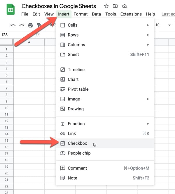
Method 1: Checkboxes are added via the Insert menu: Insert > Checkbox
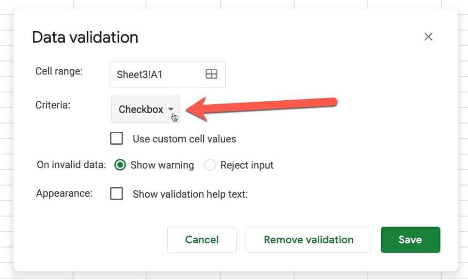
Method 2: Alternatively, you can add checkboxes via Data Validation.
Go to the menu: Data > Data Validation
And then select Checkbox from the criteria drop down menu:
Google Sheets Checkbox Notes
Google Sheets Checkbox TRUE status
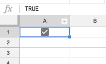
When you click on the checkbox itself, it will become checked (shown by a tick mark and grey background) and the cell value will change to TRUE.
This means you can link to this checkbox cell with any formula, for example, an IF statement, and it will behave as a TRUE value (when it’s checked).
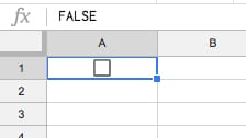
Google Sheets Checkbox FALSE status
When you add a checkbox, it will show up in the cell or range of cells that you have highlighted, and it will be unchecked. If you look in the formula bar, the cell has a value of FALSE. Again, you can use this in your formulas.
Advanced Google Sheets Checkbox Options
If you add a checkbox to Google Sheets through the Data Validation menu, you have more options.
You can set custom values for the checked or unchecked states, i.e. something other than TRUE and FALSE.
For example, see how to create a select all checkbox in Google Sheets, which uses custom checkbox values.
You can also add a validation rule so that the cell rejects any values that do not equal the values you specify for Checked and Unchecked.
Five Ways To Use Checkboxes In Google Sheets
1. Create a To Do list app
Checkboxes make it easy to create a To-Do list in Google Sheets!
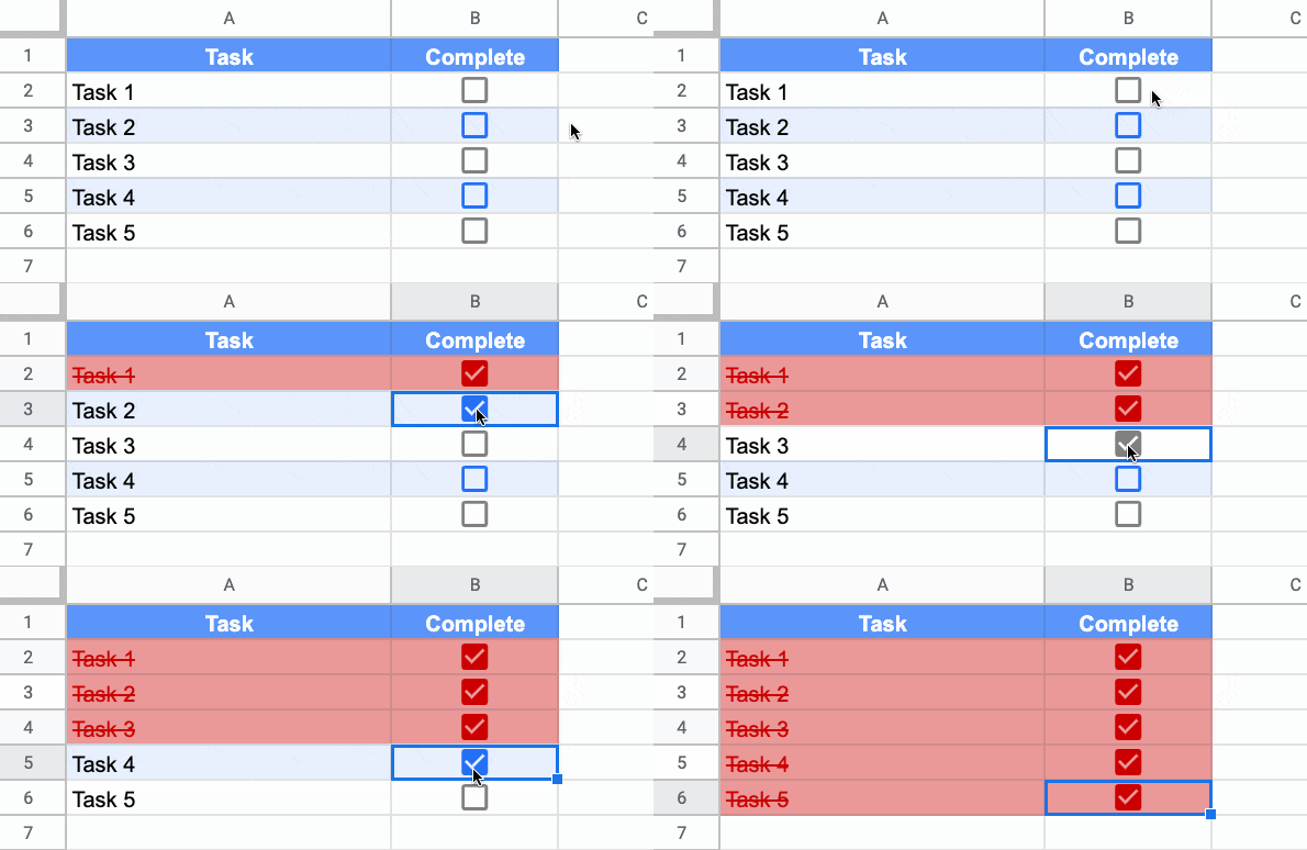
This example consists of a list of tasks in column A and a list of checkboxes in column B, with alternate colors added to the rows:

Then we can use conditional formatting custom formula rule to shade rows red when the checkbox is checked, to show that task is done.
The formula for the custom conditional formatting rule is:
=$B2The key point to note is the $ before the B only. That ensures that only column B is considered for the test but the formatting is applied to the whole row.
For a more sophisticated to-do list app, which includes a progress bar, see this checklist template here.
2. Highlight Data With A Checkbox
The same technique used in the to-do list example above can be used to highlight data in a dataset.
It’s conditional formatting applied across the row, but toggled on or off by the checkbox:
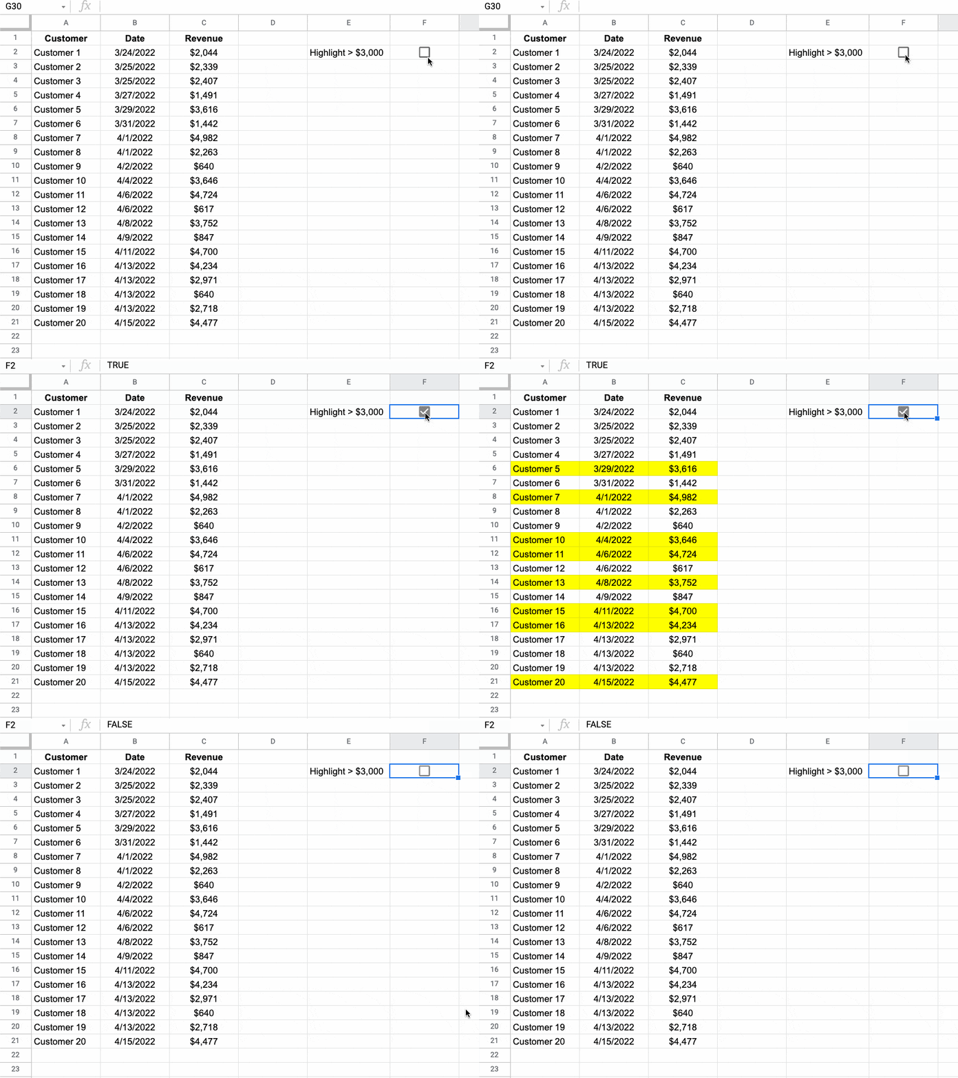
The custom formula in the conditional formatting checks that the checkbox is checked (TRUE) in addition to any other criteria.
Setup
Highlight your data range, in this case A2:C21 (omitting the header row).
Then go to the menu: Format > Conditional formatting
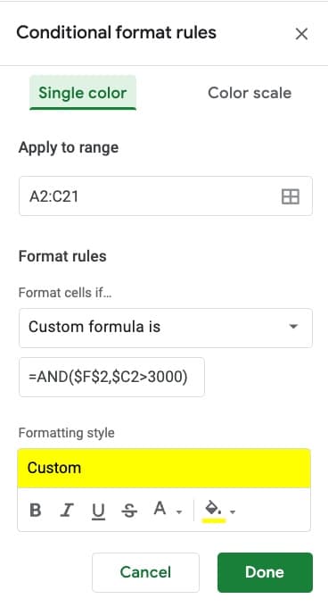
Under Format rules, select Custom formula is
As shown in the example above, to highlight rows where the revenue is greater than $3,000, enter this formula:
=AND($F$2,$C2>3000)This is applied to the range A2:C21. The $ signs ensure the checkbox is referenced correctly and that the test is only applied to column C.
The AND function ensures that the checkbox is checked (i.e. TRUE) and the criterion is met before applying conditional formatting.
Your conditional formatting sidebar should look like this:
For a second example, suppose you want to highlight rows less than or equal to $1,000. Use this formula to do that:
=AND($F$3,$C2<1000)See also how to highlight the top 5 values in Google Sheets for another example of conditional formatting. It could be combined with this AND function and checkbox technique too.
3. Show/hide hints and solutions to a test
Here's an example that may have applications in the Ed-Tech world.
Suppose you create worksheets that students use to answer questions.
Using checkboxes, you could add hidden solutions or hints, that only show when the checkbox is toggled.
Here's a simple example to illustrate this:
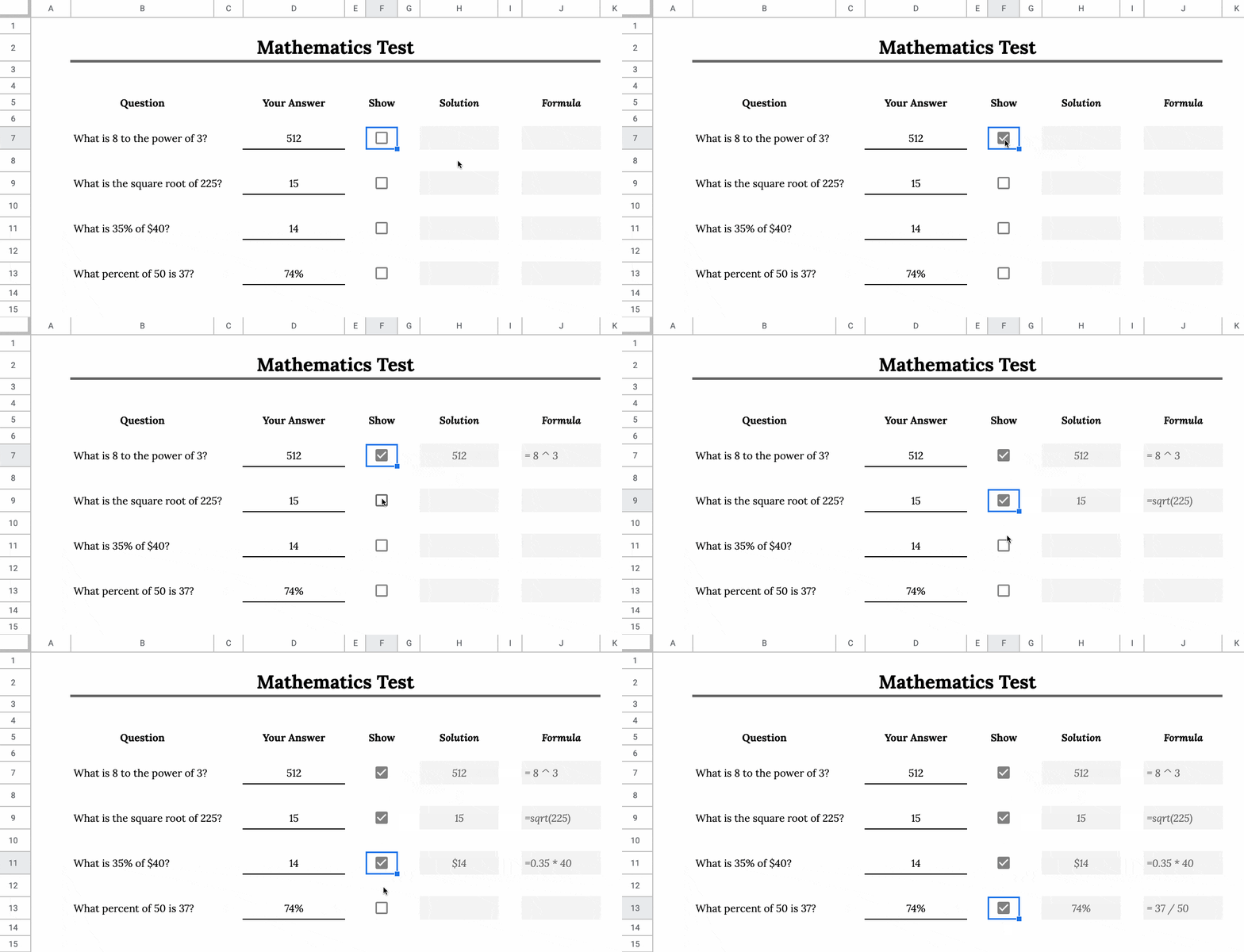
To show a hint or solution, you can use an IF function and the TRUE/FALSE value of the checkbox to show/hide the solution.
For example, with a checkbox in cell F9, the solution for 35% of 40 could be shown by this formula to show the answer:
=IF( F9 , 0.35 * 40 , "" )And if you wanted to show the formula itself as a hint, you could wrap it in quotes to turn it into a string value:
=IF( F9 , "= 0.35 * 40" , "" )4. Create dynamic charts
I've previously shown one method of creating dynamic charts using Data Validation, which works great but has the principal drawback that you can't select multiple items from the drop-down menu.
Checkboxes can solve this for you and allow the viewer to pick and choose all or any of the data series to show in a chart, as shown in this Gif:
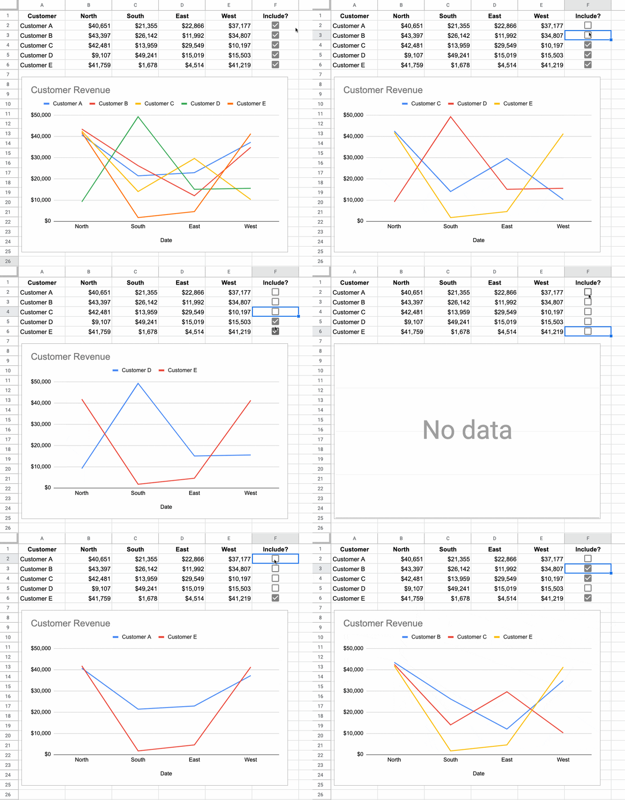
Each row has a checkbox so that a user can select whether they want to include it or not.
In other words, the data range has a column of TRUE/FALSE values, where TRUE indicates that you want to include these rows and FALSE indicates that you do not want to see these rows.
Next, you use a formula to filter out rows that have a FALSE value and create a table of data for the chart.
There are several ways to do this, including the QUERY function and the FILTER function.
For example, here's the QUERY formula to filter out the unchecked rows.
=QUERY( A1:F6 , "where F = TRUE" , 1 )The chart is then drawn from this second, dynamic data table. When you check or uncheck rows of data, those series will show or disappear from the chart.
5. Use Checkboxes As Control Switches
Suppose you have a large number of complex calculations, and your Google Sheets runs slowly because they recalculate every time you make a change.
Use a checkbox to act as a control switch and prevent these formulas recalculating all the time.
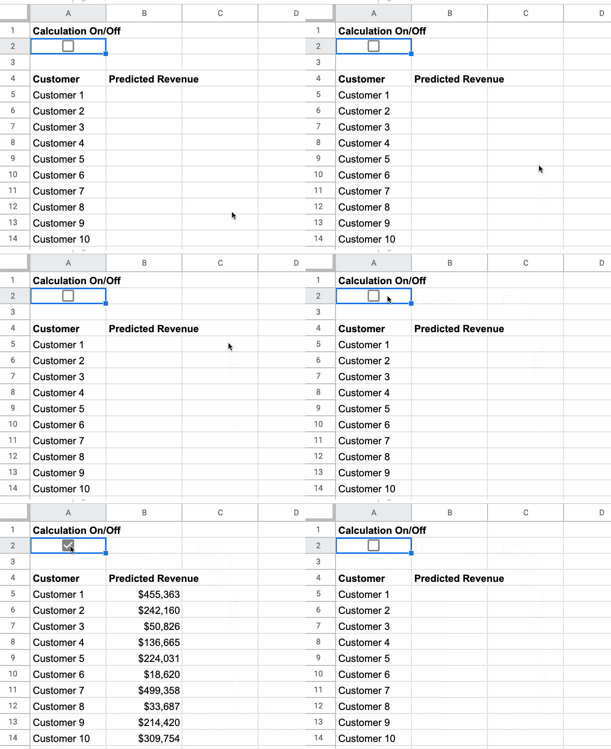
Then use an IF formula to control whether the performance-hungry formulas in your slow Google Sheets calculate or not:
=IF( $A$2,your_formula_here, )The FALSE argument of the IF function is shown blank in this example, but could be replaced with a note, e.g. "On hold".
FAQs
Q: Can you create a select all checkbox?
A: Yes, with a bit of effort, you can. Here's how to create a select all checkbox in Google Sheets.
Q: Can you make the checkboxes behave like radio buttons?
A: Yes, you can using Apps Script. Here's how to create Radio Buttons in Google Sheets.
If you want to avoid Apps Script, you can still mimic radio button behavior with formulas and checkboxes.
Checkboxes In Google Sheets Template
Click here to open a view-only copy >>
Feel free to make a copy: File > Make a copy
If you can't access the template, it might be because of your organization's Google Workspace settings. If you right-click the link and open it in an Incognito window you'll be able to see it.
That’s awesome news, Ben!
I noticed that the recording of macros has also been added to Sheets! Can’t wait to dig into this!
https://blog.google/products/g-suite/think-macro-record-actions-google-sheets-skip-repetitive-work/
Yes, the addition of Macros is great news! Hoping to have a post on here in the next week or two 🙂
Here’s that post on Macros for anyone looking: https://www.benlcollins.com/spreadsheets/google-sheets-macros/
now its ; instead ,
for example
=IF( D2 ; “checked” ; “not checked” )
Ben,
Can these be added/modified with Apps Script yet? I’m guessing the validation builder?
I’m also looking if this is possible already
I just attempted getDataValidation on a checkbox cell and received “We’re sorry, a server error occurred. Please wait a bit and try again.”, however, the same code works perfectly on any non-checkbox on the sheet.
function myFunction() {
var ss = SpreadsheetApp.getActive().getSheetByName(‘test’);
var cell = ss.getRange(1,1);
var rule = cell.getDataValidation();
if (rule != null) {
var criteria = rule.getCriteriaType();
var args = rule.getCriteriaValues();
Logger.log(‘The data validation rule is %s %s’, criteria, args);
} else {
Logger.log(‘The cell does not have a data validation rule.’)
}
}
Don’t know if you’ve figured this out yet, but the checkbox state is linked to the value of the cell it’s in. So to set a checkbox to checked, set its associated cell to true or 1. Alternatively, using data validation in the cell you can set the checked/unchecked values to whatever you want. To change the status of the checkbox just change the cell to the appropriate value. For example, I have a checkbox set in the data validation menu to checked = 25 and unchecked = 0. I can make it checked or unchecked simply by doing this in a script.
SpreadsheetApp.getActiveSheet().getRange(“Sheet1!N19”).setValue(25);
or 0.
Any idea on how to dynamically select a checkbox based on a value of another?
eg =IF( G8 <=10, TRUE, FALSE )
If TRUE checkbox is selected, if FALSE Checkbox is not selected.
It seems when setting the boolean values TRUE or FALSE overwrites the checkbox cell.
You can have that formula in a cell to give you the TRUE/FALSE value, but you can’t also have a checkbox showing.
The checkbox is actually a data validation on the cell, so if you type TRUE/FALSE (which will delete the formula) then the checkbox shows again.
Cheers,
Ben
Ben please, I have created a Google sheet that have several protection on it I want a script that duplicate the sheet protection with the sheet anytime I duplicate it.
When I look at the insert menu or the data validation criteria I don’t have the option for checkbox. Is there something I need to do to enable it?
Samantha: I’ve notice the same. I use two browsers, one in English and the other in Portuguese. There’s the new feature in the english one. Maybe in some time we’ll have it in all of them.
Hi Samantha,
As Gilmar mentioned, I think that the feature hasn’t rolled out to everyone yet. I’m sure it will do soon though.
If you’re a G Suite customer, you can select to get new features on the rapid release track: https://support.google.com/a/answer/172177
Cheers,
Ben
Ben, thanks for alerting about this new awsome feature! I have used it instantly on a Google Sheet of pay bills to indicate already paid/not yet paid bills w/conditional formatting.
Great tip!
Great stuff! 🙂
Is there a way to make the checkbox have a third state? Like, unchecked, checked, and x? Thanks!
There’s no third state but you can still type whatever you want into the cell, and override the checkbox. However, you’ll see a “Invalid:
This cell’s contents violate its validation rule” error message.
The TRUE/FALSE checkbox comes back if you type TRUE or FALSE again.
Hope that helps!
Ben
I would also like the option to have a third state on checkboxes if possible down the road. Yes (check)/No(x)/Blank (=unanswered) would be awesome and useful functionality. When logging data, it helps to know which is affirmatively negative and which just hasn’t been answered/entered yet.
That is really cool, but I don’t think it has been rolled out to all users yet. The option doesn’t appear for me on my grandfather-in g-suite account, or on my more recent company account.
Hey Jesse,
Yes, you’re right. As of early May, they haven’t rolled out to everyone yet but they should be available soon.
If you’re a G Suite customer, then you can select to go on the rapid release track which will make them available: https://support.google.com/a/answer/172177
Cheers,
Ben
This is just what I need for my latest project. Do you know if it is available to dynamically add through the api? I can’t see it in the docs.
Great question! Not sure either, as I couldn’t find it in the docs when I looked. I’m sure it will be available in time though.
Ben
Hello Ben,
Very nice article and examples. However, when I try to use the =IF(A1=”TRUE”,”YES”,”NO”) in order to insert in B1 a “YES” if my A1 is checked it says “Formula parse error.”. Can you help me with this please? 🙂 Thank you in advance!
Hello,
try to lose ” in formula. Worked for me. 🙂
=IF(A1=TRUE,”YES”,”NO”)
Hey Lucian, Roman,
You can go one further and actually just ditch the comparison with TRUE, since if A1 is TRUE the IF statement will execute the TRUE part of the logic. i.e. your formula could be even shorter:
=IF(A1,"Yes","No")Cheers,
Ben
Hi Ben, any thoughts on using a countif on these? Looking to use this for process management where 1 piece of inventory has 3 or 4 different checkpoints and the countif would allow me to create a dashboard/scoreboard for that process completion.
Figure this out yet?
Hey Mitch,
Yes, you can use COUNTIF. For example, suppose you had your checkboxes in column A1 to A10, then this formula will count whenever they are checked:
=countif(A1:A10,TRUE)Cheers,
Ben
Hi
Just tried the new Checkboxes (could make many of my spreadsheets cleaner), but hit an issue.
If you set up cells with checkboxes, and CLEAR the cell content (select sell, hit delete) then the checkbox doesn’t un-check, but disappears entirely! That makes it pretty much unusable, as most users will use that method to clear a check.
Is there anyway to prevent if from being deleted?
I am looking for a solution to that exact same problem as well as the ability to add these back (onOpen) through AppScript. If users delete the checkboxes (as most certainly they will), this destroys any reporting applicable to that cell. I cannot seem to find a solution out there for either? Any suggestions welcome!!!
Hey Ian,
Unfortunately I don’t think there’s a way around this at present…. If I find any “hacks” I’ll post them here.
Cheers,
Ben
Utilizing the checkboxes for a selection of cells (i.e. 5 of them), is there a way to limit that selection of cells to only allow ONE checkbox?
You can merge those 5 cells and then insert a single checkbox! 🙂
Hi Ben,
I hope what Brain is asking for is – out of 5 Checkboxes, the option we should have – is to check only one Checkbox.
Incase we check another check box, the earlier checkbox should be unchecked automatically.
He is looking for an option what we have in the Google Forms.
thank you
This is a great functionality, but there is a problem with it: users can delete it. If you have an editor allowed to edit a range, that person can delete the checkbox. So this not a good functionality to be shared, yet.
You can easily protect those cells to restrict the users to delete those.
that’s an option depending on what you need to share. If you need users to use this checkbox, if you protect the range, they will can not interact with it. It is kind of weird, you can set a data validation in one cell and users can not delete it, but if you use the checkbox it can be deleted.
This is also my problem in using checkboxes, I want to prevent other users from removing/deleting the checkbox itself, but also they can interact with it.
Hi Ben,
When using Forms to populate the Sheet, is there a way to have the form answer cause a check box to be checked? So for example, if on the form I ask “what is your favorite food?” and you check “steak” out of a possible 6 choices, right now “steak” shows up on the sheet as text. Can I have that response automatically click the Steak Checkbox that I created in the same row (assuming I create a series of checkboxes tied to the possible responses)? Thanks
Hey Greg,
Unfortunately I don’t believe this is possible at present, at least not with formulas. If and when checkboxes are accessible with apps script, it might be possible to achieve this then. I’ll keep an eye on the reference docs and post an article once we can access checkboxes with apps script.
Cheers,
Ben
Great Article. Was able to use it to conditionally format cells based on the check marks. One issue I had is that if I tried to set the rule for more than one cell with a checkbox I could not do it. Is there any way to do this. What I want is to have several checkboxes and if all of them are unchecked I want it format it one one while if one of the checkboxes is checked it formats it another way.
Hey Joshua,
Without knowing the precise details, you should be able to achieve what you want by using the AND and OR functions, and maybe some IF statements…
Basically, the one scenario you mentioned is equivalent to:
FALSE | FALSE | FALSEin your cells.
Hope that helps!
Ben
Is there a way for only one checkbox to be checked at a time in a range of cells? So if someone checks one box it unchecks the other one selected in that range.
Hey Scott,
Unfortunately not with these checkboxes. They exist independently in their cells so you can’t create a multiple choice. Best way to solve this is to create a drop-down menu using data validation as this forces a single choice.
Cheers,
Ben
The workaround I have found for this is to utilize a script like the one below. Basically, it checks that the box I’ve marked is now “True” (i.e. it’s value is “1”) and, if so, it clears the contents of all other checkboxes in that group; in this case, all my checkboxes are in the same row:
function onEdit(e) {
var test = SpreadsheetApp.getActiveSpreadsheet().getActiveSheet().getName();
var s = SpreadsheetApp.getActiveSpreadsheet().getSheetByName(“Song Database”);
var row = e.range.getRowIndex();
var col = e.range.getColumnIndex();
var c = s.getRange(row,col).getValue();
if(c == 1 && col==4) { /Song is ready/
s.getRange(row,5,1,3).clearContent();
};
if(c == 1 && col==5) { /Song is a work-in-progress/
s.getRange(row,4,1,1).clearContent();
s.getRange(row,6,1,2).clearContent();
};
if(c == 1 && col==6) { /Song is homework/
s.getRange(row,4,1,2).clearContent();
s.getRange(row,7,1,1).clearContent();
};
if(c == 1 && col==7) { /Song is proposed/
s.getRange(row,4,1,3).clearContent();
};
};
Thanks for this, its really helpful, however am getting the below error, any idea how this can be fixed
TypeError: Cannot read property ‘range’ of undefined
Is it possible to gain access to the spreadsheet referenced in “1. Create Dynamic Charts” that explores using checkboxes to show/hide data in a chart of GDP by country?
I’m trying to play around with a similar feature and I think it would help to make a copy of your Sheets example to explore.
Thanks in advance!
Hey Joey,
Here you go: https://docs.google.com/spreadsheets/d/1ASd33HVq7c_8bDsXUUV-3oQ7oIrOSXLzJrYk_QjHrzY/edit?usp=sharing
Cheers,
Ben
Hi Ben
Do you know how you can create a “Check All/Uncheck all” box? I know you can do this in excel but can’t figure it out on G sheets.
Thanks
Athena
Hey Athena,
Unfortunately you can’t do that at present with these checkboxes. They’re independent of each other. I think we’ll see more functionality in the future though.
Cheers,
Ben
Macro or scripting does it easy running from Script Editor 🙂
Now I have to find a way to fix this error when running from spreadsheet: “You do not have permission to call setValue…”
Cheers!
Is there anyway to link the check boxes so if a box is checked on one active sheet it automatically copies to another sheet in the same document – I want to use them for attendance records each teacher has their own tab and I’d like to have a copy of everyone’s data on a final tab using a copy function.
You could have a checkbox link to another cell, which would display the same TRUE or FALSE value, but you can’t link to another active checkbox.
Cheers,
Ben
Sorry, but do you mean you can’t have it linked to another active sheet?
Hello Vicki! I have I think the same kind of question! Did you manage to to do this?
I’ve got curriculum standards in a column. If it’s checked in another column, I want that standard to be copied to a particular sheet. https://youtu.be/SPiILUaOKYo
Hi,
Can you add a conditional format so that when you untick a checkbox it will remove the cell colour. I can do it so the cell turns a different colour when i check the box but not when I uncheck it.
Regards
Hi Todd,
Sure. You can set a conditional formatting rule for when the cell value is FALSE e.g.
Thanks,
Ben
I have 4 checkbox options in a row to track the workflow of a document. A2=checkbox for “buyer signed”; B2=checkbox for “seller signed”; C2=checkbox for “completed”; D2=checkbox for “N/A” (document not needed in this transaction).
I tried conditional formating so that if the checkbox C2 is selected, A2:B2 would gray out, and adding a second conditional formatting for if D2 is selected (N/A) that A2:C2 (or the entire row) would gray out. Anytime I add the 2nd conditional formatting formula, it deletes the other. Is there a reason for this? It doesn’t seem to want to allow both to exist together.
Hey Luke,
Hmm, not sure why they’re being deleted… If you mean they’re not working as you expect, try changing the order of the rules (you grab the rule handle and drag it above the other one). The rule at the top will take priority over those below.
Hope that helps.
Ben
Hey there. I’m trying to have one cell add up cells A3:A50 and that worked fine using the SUM function. However, cells B3:B50 have the check mark box next to them. Is there a way to have the SUM function only add the numbers whose corresponding check mark box returns a FALSE value? I’m trying to figure it out but I can’t seem to not get errors.
Hey Allan,
Yes, you can do this using the SUMIF function, like this:
=sumif(B3:B50,TRUE,A3:A50)Cheers,
Ben
I’m trying to figure out the data validation to use so that if the word “admin assistant” is found in a cell, it checks the box; however, the cell could have “admin assistant”, “HQ”, or “Evang admin” in it. Is there a way to check a box in E2 if “admin assistant” is in the cell D2, check the box in F2 if “HQ” is in the cell, and check the box in G2 if “Evang admin” is in the cell?
THis is great, thank you. I have a sheet with 50 or so rows and 10 columns. Each cell is a checkbox that corresponds to a step in a process. How can I apply the formula you used for the color change ( = $B2 = TRUE) en mass so that each individual cell is independend to each other?
i.e. rather than change the color of the whole row, I just want to change the color of each individual cell.
Thanks in advance.
Hi Martin,
Change your conditional formatting rule for the whole range (all 50 rows and 10 cols) to be:
Format cells if…
Is equal to
TRUE
Cheers,
Ben
So when can we activate a Macro with the check box?
Is it possible to Hide / Unhide a sheet based on a checkbox?
Hi Ben!
Late to the game and I’m slowly learning 🙂 Your site is helping me tremendously so far!
I ran into a mini issue and I’m not really sure if it’s possible to do or not. Can’t find anything but I might not be using the correct terms. I’m making a sheet with client’s payments that didn’t go through. Once I have their updated billing info I’d like them to “fall” down to the bottom of the list once I “check” off this box. Is there anyway to do this?
Thanks so much,
Dani
You could use a filter on that column, just showing the False ones, and the true ones would be hidden.
Ben
I am loving your videos for Data Studios, absolutely fantastic.
I am having a issue which searching for via the forums, doesnt seem to have an answer for.
In my google form I have check boxes, which creates multiple answers in a cell. When I then create a pie chart, it doesnt seem to treat the multiple answers, as individual answers. Is there a way around this?
Question: I am using check boxes for meeting students. So, I was able to put a rule where if I check the checkbox, it automatically turns green. But, I really need the whole row (not column) to turn green when the check box is pressed. Is this possible? If so, how?
Thanks in advance.
Hi Angelann,
Yes, you can definitely do this. Have a look at the conditional formatting custom formula rule that I apply in the To-Do app section of this article.
Cheers,
Ben
I am trying to find a way to have an uber list that I can check values I want and have that spit out a list of only those values. That way I can generate different specific tasks for different project. Any thoughts on how to do this?
Oh! I figured it out using your example for the chart. Duh!
I was going to use this to track data with my students. Is there a formula I can put at the bottom of my column to count how many boxes are checked?
Thanks
Hi Kelly,
Yes, you can use a COUNTIF formula to do that! Have a look at this comment: https://www.benlcollins.com/spreadsheets/checkboxes/#comment-64226
Cheers,
Ben
Thanks for this! Really useful info. Is there a way to use checkboxes on a published google sheet?
Hi Ben,
i want to add macro checkbox. how can i do that? i recorded a macro. i want to run this macro with checkbox. i write a cell =myFunction() then i take this eror ” You do not have permission to call setActiveSheet (7. satır).”
My Macro
function myFunction() {
var spreadsheet = SpreadsheetApp.getActive();
Utilities.sleep(2);
spreadsheet.getRange(‘U2’).activate();
spreadsheet.setActiveSheet(spreadsheet.getSheetByName(‘Yapılan işler’), true);
spreadsheet.getRange(‘A3’).activate();
spreadsheet.getRange(‘Planma!U2’).copyTo(spreadsheet.getActiveRange(), SpreadsheetApp.CopyPasteType.PASTE_VALUES, false);
spreadsheet.setActiveSheet(spreadsheet.getSheetByName(‘Planma’), true);
spreadsheet.getRange(‘B2’).activate();
spreadsheet.setActiveSheet(spreadsheet.getSheetByName(‘Yapılan işler’), true);
spreadsheet.getRange(‘B3’).activate();
spreadsheet.getRange(‘Planma!B2’).copyTo(spreadsheet.getActiveRange(), SpreadsheetApp.CopyPasteType.PASTE_VALUES, false);
spreadsheet.setActiveSheet(spreadsheet.getSheetByName(‘Planma’), true);
spreadsheet.getRange(‘C2’).activate();
spreadsheet.setActiveSheet(spreadsheet.getSheetByName(‘Yapılan işler’), true);
spreadsheet.getRange(‘C3’).activate();
spreadsheet.getRange(‘Planma!C2’).copyTo(spreadsheet.getActiveRange(), SpreadsheetApp.CopyPasteType.PASTE_VALUES, false);
spreadsheet.setActiveSheet(spreadsheet.getSheetByName(‘Planma’), true);
spreadsheet.getRange(‘F2’).activate();
spreadsheet.setActiveSheet(spreadsheet.getSheetByName(‘Yapılan işler’), true);
spreadsheet.getRange(‘D3’).activate();
spreadsheet.getRange(‘Planma!F2’).copyTo(spreadsheet.getActiveRange(), SpreadsheetApp.CopyPasteType.PASTE_VALUES, false);
};
Hi, I have a problem which I’m hoping someone can help.
I have 4 columns (A-D) with tick boxes using the tick box function on sheets. I wanted to put a formula in so that if I select column A as True then it will automatically select columns B-D as true (tick the boxes). I got this to work with IF formula, however I’m then not able to untick or use the tick box in columns B-D as if has the the formula in the cell.
Any Ideas?
A B C D
All John Jack Steve
TRUE IF(A2=TRUE,TRUE,FALSE)
I am using the checkboxes as a completed task check. They are both in separate columns. Is there a way for me to format it so that the row changes color based on both boxes being checked?
I´m wondering the same thing and would very much like to know.
Anyone know if you can have mutiple checkboxes inside of a single cell? As an example, we are using a google spreadsheet to house content for “Projects” (up to 100 projects).
Each project consists of data points such as:
– Completion date
– Project name
– Project Summary
– Related Market Sectors (this is where I would love to have a cell allow for someone to checkoff multiple “sectors” and ideally these would all live inside of a single cell as each association of a sector for each project is unique to each project).
Any help/insights would be greatly appreciated!
I don’t think this would be possible since the checkbox sets the value of the cell (Usually as true or false). You can’t have more than one value in the same cell.
Thanks, Samantha! Yes, you’re correct. Only one checkbox per cell so you’ll have to work with that.
Ben
You can, although I think you have solved this. Nested If’s
=if((AND(H30,J30,L30,N30)), “Pass”, “Fail”)
and I have checkboxes in there
Hi Ben,
Thanks for the great article.
I’m having a problem with checkboxes that I’m sure you can help with:
When I copy a spreadsheet with checkboxes into another sheet using IMPORTRANGE, I lose the formatting. I “solved” this by simply inserting the checkboxes manually into the new sheet, which seemed to work fine. However, when I share the second sheet with someone else, the boxes appear empty, though the text in them is correctly “TRUE” or “FALSE”. Anyway I can share the second sheet without this happening?
Thanks!
Is there any way to turn these into radio buttons? Like when one is checked the other boxes automatically are unchecked? IE Only one can be checked at a time.
Unfortunately not. They’re all independent, and just toggle between True/False states.
Ben
https://stackoverflow.com/a/59233129/9471761
Is there anyway you can alter the condition of the check box based on the results of another cell?
i.e. If a list of items is blank ( nothing selected/ cell empty ) the checkbox is false, but if something from the list of items is selected the checkbox is true?
Hello,
My question is similar to one posted above.
I’m very new to google sheets and do not have experience with excel. I have columns on an invoice with checkboxes. The checkboxes are used for contractors to check if the fee they are billing for
is for labor or materials. When I view the sheet, I see the checkboxes. I am able to edit and create a check mark in the box. However, when those who are granted access to edit via shareable link view the document, they see the words “true” or “false” If they click on them they change from “true” to “false or vice versa. I would like for them to see only the boxes, and be able to place the checkmark. Thanks!
Has anyone noticed how adding the new checkboxes extremely slows down the opening and processing of a google sheet?
I am using the check boxes for planning a wedding–checking the boxes of who received an invitation to the wedding, the shower, etc. Is there a way to add how many boxes I have checked. I would like a total at the bottom saying I have 38 boxes checked.
It is a great development but I wish they would link better with excel. The company I work for is using both sheets and excel so I need a form with interchangeable functionality. However, a check box in sheets comes through as true/false text when downloaded to excel, yet in sheets they show as an image when importing an excel version that cross over the text options. I have to have two different versions of a form to accommodate those who’ve moved over to sheets, but it’s proving a nightmare when the form crosses over!
I can’t even think of a way around for selecting an option without a tick box or form control, only to maybe ask the respondent to highlight their option in bold or something, which totally negates the ease of a check box! Any suggestions?
The only thing that differs between Excel and Sheets on checkbox is the separate image in Excel. In Sheets, image and TRUE/FALSE are on the same cell. Also, Excel takes 3 values: TRUE/FALSE/NULL.
The good news is, they both react to TRUE/FALSE cell.
Simply create extra import/export tabs for each so they’ll be compatible. Meaning in Excel, have separate tab that will be compatible with Sheets and vice versa.
I hope that helps – Cheers!
Hi,
I am new to google sheets. I have worked out how to add up how many boxes are checked using Countif.
Is there anyway to work out what the total percentage of boxes that are checked in the row?
eg. if 4 out of 8 boxes are checked – it would be 50%
Thanks
Hey Bek,
Yes, you can add a COUNTA to get the total number of checkboxes as your denominator. For example, if you have 10 checkboxes in A1:A10, this formula will determine the percentage that are checked:
=countif(A1:A10,"true")/counta(A1:A10)Cheers,
Ben
Thank you!!
Hi,
I’m adding rows into a sheet using the sheets api (interacting through integromat specifically). Is there any way I can add a checkbox into a couple of cells in the row. A checkbox doesn’t copy with a function.
Right now I can only do that by copying from the previous row.
Thanks
Thanks for sharing this Ben, those graphs option are very helpful. Could be the next enhancement to my existing Sheets.
Looking forward to Radio Button function too, where you can only select one from the options. Normally in circle buttons but I won’t mind the tickbox as long as only one option can be selected.
Also trying to find ways to show checkbox without scripting when another cell is not null. I need the checkbox to show only on column B for example, when column A have value…
Hi Ben,
I have grouped rows together and the first row is a header for a list of tasks that need to be done for a project. Can I check the main task/header as complete and subsequently make its sub-tasks marked as complete automatically?
Thanks!
I’m trying to make every checkbox checked to add 3 to a total value (almost like shopping) but not really sure how?
Hi and thanks for all the great information provided on the blog the courses.
I´ve got a question regarding checkboxes and conditional formatting.
I have a row with 5 checkboxes. I know how to apply conditional formatting so that the entire row changes depending on if a checkbox is checked or not.
Now, how would I go about if I want the entire row to change (nackground color for ex.) if all checkboxes are “checked”.
I´ve read through the comments and I have tried with the best of my abilities, but without any luck,
=IF( AND( firstcell=TRUE, secondcell=TRUE, … lastcell=TRUE))
or
=COUNTIF( rowrange, FALSE)=0
or several other ways.
Hey Ben – I am trying to create some if/then formulas off of the checkboxes, but it doesn’t seem to work. This is the basic idea of my formula – =if(C75 = “TRUE”, “YES”, “NO”), and no matter if the box is checked or not, it always populates “NO”, as if it doesn’t recognize the “TRUE” or “FALSE” that populate the referenced cell, C75. Any ideas on this?
TRUE and FALSE are Boolean conditions, not text. Remove the first set of quotes, and it will work.
=IF( C75=TRUE, “YES”, “NO”)
Or make it even simpler than that. The spreadsheet software evaluates the condition to arrive at an answer that is either TRUE or FALSE. If C75=TRUE, then all you really need is
=IF( C75, “YES”, “NO”)
Hi Ben,
I’m using these for a to do list/task management for my team and was wondering if it’s possible to format so that if a box is checked, the entire row is moved to another tab that I would call “Completed”. I’ve been just moving completed tasks myself or filtering but it would be great if I could get it to do this automatically. Thanks!
Is there a way to link the data such that I have a master sheet and individual data sheets and if I check the box on the individual data sheet it applies the check and conditional formatting to both the individual data sheet AND the master sheet?
Found this via Google search for “radio button Google docs”. I still wish there were an out-of-the-box solution — BUT — your To-Do list example helped me achieve the intended function with a useful, elegant workaround. Thank you!
You’re welcome! That’s great. Thanks for sharing.
Ben
Hi Ben,
I was wondering if you can help, if I have a list of names in a sheet and selection of tick boxes for each name (in this case vehicle types they are licensed to drive) Is there a formula I can use to copy their names to a different sheet within the same doc based on the status of that tick box?
Thanks
Hi!
I have a sheet that i want to record my time i work in.
At certain times i work overtime and have different paygrades on the time. What i want to do is to have a checkbox to tell the sheet if the overtime is approved or not and then it calculates the diffrent times into different columns. If not approved i want everything in one cell at that column.
Hard to explain but it’s a simple setup.
Anyone have an idea what to do?
There are 3 cells that need to read the checkbox and do one or the other depending on true or false.
Here is a link to a test document.
Some words are in swedish 🙂
Övertid = overtime
Mertid = overtime with out extra pay
Need the Övertid checkbox to be ticked and then fill the extra pay columns (first the 16:00 one and when time passes 20 (8 pm) then fill that column with the time after 20.
Here is a link to the test document 🙂
https://docs.google.com/spreadsheets/d/1G4zV0RYTFj06RYssc9oXGAAggqLziYTwylfKX4Ttvjw/edit?usp=sharing
Thanks!
Got it solved! 🙂
Is there a keyboard shortcut to check and uncheck a box?
Great question! Yes, pressing the spacebar will toggle the checkbox check/unchecked.
I want to add a completion checkbox at cell c68 getting all checkbox from c5:c67 to be true. I was hoping this might work: =IF({C5:C67},”COMPLETED”,””) however it shows completed even thought a cell example c5 is unchecked. Please any advise on this project.
This should be easy, but I am missing something…. I created a Query to extract data from main sheet into a secondary sheet. However the CHECKBOX (Column F) becomes TRUE or FALSE. I tried Data Validation and that made my query information disappear. Can the desired result be built into the Query formula? If yes, suggestions…
=QUERY(Sheet1!A:G,”select A,B,C,D,F,G where E=’AHS ‘”,1)
The checkbox looks great. I would like to format data with a checkbox, but the checkbox is formatted data and a built-in ui.
Checkbox registers as data, 1 or 0 (true/false).
If a checkbox is added to the cell, it is considered a cell with data. ISBLANK returns 0.
Now I have an array formula returning true or false (1/0) and I would like the results displayed as a checkbox.
my function:
(A2:A) == 100? 1 : 0
I would like to display this as checked and unchecked boxes.
Hi Ben, really cool work!
Do you think is possible to make a progress bar or a dynamic chart with checkboxes?
I mean if I have 100 checkboxes, and I check 50, a chart o progress bar that shows the percenteage 50% or the progress like 50/100 of checked boxes.
Thank you in advance
Hi Ben,
This is a great post. Thank you for writing it.
For checkboxes, is there a way to have a person be able to select only one checkbox. I have a checkbox for Yes, No, and N/A (as part of a scoring rubric). If a checkbox is selected for “Yes”, the person shouldn’t be able to select the checkbox for “No” or “N/A”.
Is that possible?
Thanks in advance!
Ben, it’s wonderful that you continue to create these very helpful posts!
I have a single question re the use of the checkbox.
I have one column on a google sheet that teachers can select student names so that the teacher can send emails to those selected.
Is it possible to make the checkboxes interactive on a new google site so that the teacher can use a web page that has the sheet instead of the sheet itself?
Thank you very much!
Are you able to assign the checkbox to a number so when you enable your column of checkboxs, it will have a sum total of the assign number?
I’ve try it with a column of number and a column of checkbox beside it and had “=SUMIF(I24:I27, TRUE, H24:H27)” as the total. but I don’t want my number to show in a column, don’t know if there’s another way?
Hi Ben, hello to all the fans of Google Sheets!
Let me show you something I did with the check boxes.
To color a Gantt diagram I used conditional format for the boxes, between true and false, color on color for true and white on white for false (this is not conditional)
Google Sheets does not allow check boxes to have color and contrast of the exact same color. To avoid that restriction I used two very similar colors playing with RGB, for example # FF99CC on # FF99CD, these are two different colors for the restriction, and for the eye they are practically the same.
I leave a copy of the sheet where I applied it, I hope it is useful. Click on each box in the diagram!
https://docs.google.com/spreadsheets/d/1dFBSFQ2SLqRGBvzSmTC2C7dWWaMd3kBix5Q0EmdHPFc/copy
Greetings to all!
Raúl, from Buenos Aires.
Nice work, Raúl! That’s a neat trick and your Gantt chart sheet looks really smart. Thanks for sharing!
Thank you Ben, I appreciate your comments and your work, it is an honor to share in this space. A greeting.
Hello, I have question.
If i apply the data validation for the entire row/column but only to make the drop down availble when the next to it column have value, how is it?? is there any extra formula? because the drop down will appear even there is no data next to it.
Hi Hsak, I think that this form of custom formula should work in the conditional format of the row:
=AND(($E6=TRUE),($D6>10))
I hope it is useful, greetings.
Raúl
Hi Ben, I want to insert a checkbox in a google sheet using a formula. So for example if cell A1 is not NULL then I want to insert a checkbox in cell B1. Is there a formula or a script that could do this please?
Something like =if(A1″”, “CHECKBOX???”, “”)
Kind regards,
Angel
Unfortunately you can’t add checkboxes with formulas. I agree that would be cool though…
Thanks Ben for your reply. Ben, is it possible to add the current date/time in an adjacent cell when a user ticks a checkbox?
Good morning Ben,
I would like to know if there is an option to add a time stamp to the check boxes. Example, if someone checks it I would like it to populate the time, date and if possible the initials of when/who checked it. I know I have seen this on an application somewhere, but no idea where I saw it.
Hi. How can I use a formula that says if my check is true then sum this, don’t sum it if checkbox is not ticked?
I tried this but it doesn’t work
=IF(K6=TRUE,”YES”,”NO”),SUM(P29:P31)+’Sprint Values ‘!C2)
Dear Ben,
Thank you very much for this interesting technique regarding the creation of a dynamic chart using the checkboxes. I created a dynamic bar chart using the checkbox function. In a hidden tab, I created a query function giving me all the lines where a checkbox is marked. Basically identical to your approach but within two separate tabs. Unfortunately, when the number of checkboxes marked, falls under a certain amount, the bar graph does not display any data anymore. I found out that the setup of the graph automatically changes. It then deletes the data series and puts the number that should be displayed as a bar as a label of the x-axis instead. (which does not make sense at all) I could not manually change that, as it automatically resets. I saw that this was not a problem with the example that you shared with us. Do you have any idea why there is a difference in that? Thank you very much for your help in advance.
Hy,
Can anyone help me with smth, i was wandering if it is possible to make a script that hides some rows when a checkbox is ticked, and unhides them when the same checkbox si unticked. i have done 2 macros, Hide and Unhide, but i cant manage to link them to the checkbox. I have tried it in the script editor but cant manage to run.
Ty
Hi, Ben! Great content, as always…
Do you know if I can use the status of a checkbox to control the actions of a google script?
To make this clearer, here’s my use case:
The managers in my company have a sheet that they use as a template. Data is added to the sheet all week long, then the sheet is “reset” Friday evening with a script. But now some of the managers want to clear the sheet manually on Mondays.Can I control the “reset” script using a checkbox? (Tick the checkbox to have the script reset the sheet, or keep the checkbox cleared to leave the sheet alone.)
I can “read” the condition of the checkbox using a script to control the reset process using an IF THEN statement.
Is my idea doable?
Yes you canDo it.
Given you add a simple checkbox, the cell value will be ‘true’ or ‘false’.
Read the cell with the checkbox and
checkBox.getValue(); // will be ‘true’ when checked
This post is elder, but if YOU like reading interesting things “all the way down” (and this blog post *is* interesting) I wanted to give you my work for a Radio button set of checkboxes. It is now possible -july 2020-.
Taking the fact that if you render invisible a check box, simply by text color formatting it to white, sheets will dialog out any atempt to change it -alternate-… then all you need is Conditional formatting to hide the group of checkboxes (except for the checked one) to have a nice Radio button effect.
You need to use a cell to receive any TRUE value from the set: ie. E1 for a set of checkboxes in E2, E3 & E4
fórmula in E1… =Or(E2:E4)
Then set conditional format for E2:E4 with a custom formula: =And($E$1,Not(E2)) giving the same foreground and background colors to unchecked cells.
Great Post, thank you Ben.
I am stuck with a seemingly simple problem. How could I show a row thats set on TRUE at a different place in the sheet? https://ibb.co/8MS8KcG
Thank you for a tipp in the right direction! flo
Hi Ben,
I was wondering if you could help me with a checkbox issue, I’m making an audit form on sheets and would like to have every tenth checkbox turn red, but to re-set the formula so the next checkbox is white until the tenth box is checked again, is this possible?
Hello!
Thank you so much for this helpful information.
Is there a way to limit the ability to check a box in a column dependent upon if a box in another column is checked?
I.e., I have 2 columns with checkboxes functioning as an “either/or” choice. If the checkbox in Row 2 Column A is checked, I want Sheets to prevent the user from being able to check the box in Row 2 Column B.
Hey great article. Does anybody know how I might go about creating an export filter which only selects rows which have the false statement to another sheet or document? (For a to do or shopping list for example).
Cheers!
Can you use a checkbox to cause another cell to generate a random number? But that random number generate is ONLY tied to a specific checkbox.
IE, box is unchecked = no number, specific box is checked = random number generated
Hi Ben, I am new to Google Sheets and I am learning so much from you! Thank you!! I was wondering if there is some type of formula that I can use that when a checkbox is ticked that the date the checkbox was ticked is entered in the adjacent column?
@Tiggy, this may be what you were after. If you check box is in B5 then use this in C5.
=if(B5,TODAY(),)
If you are using checkboxes to control branching in Google Apps Script, be aware they return (weakly typed) *string* values, not Booleans:
If there’s a checked checkbox in A1, the formula
= IF(A1,”Yes!”,”No.”)
in cell B1 returns “Yes!” but when you check the cell, apps script code in inEdit()
if (e.value) {…}
will NOT execute. You need
if (e.value==‘TRUE’) {…}
To be safe, I use data validation to set checkbox explicitly to ‘TRUE’ / ‘FALSE’
If someone else has already pointed this out above, my apologies for the duplication.
hi ben,
I want to try creating table format with different colors.
But it depens on custom range. So how many records has it which table has to be records of row.
For example; A4 cell has a dynamic value and table must be colored range max A4 cell.
you know Google sheets has no custom area value, How can we use custom area value?
Hi,
Is there a way to duplicate information from an entire row in one spreadsheet to another using a checkbox please?
Hay
Can you tell me that, Is there any option to shift to entire row with information From sheet3 to Ready for delivery sheet using checkbox ?
Found it very useful but wish one thing would have been covered.
Like to know how to make it if any checkbox is checked the others get unchecked. Spent hours trying and failing to do make it work.
I have a list of names and I wanted to create a checkbox to randomize the list as a shortcut to highlighting the list and then going to Data then randomize range, is this possible?
I have this table that works fine, but I have a problem when I want to apply filters.
I would like that when I filter column A, in cell D2, not to calculate the rows that are hidden by filtering (A kind of SUBTOTAL()). Can someone help me with an idea?
A | B | C | D | E |
Number | Amount |Collected| SUM | formula |
————–|—————-|————-|————-|—————————————–|
22SSS | 100 | TRUE | 100 |=sumif(C2:C;true;B2:B) |
55SSS | 50 | FALSE | |
44SSS | 50 | FALSE | |
33SSS | 1 | FALSE | |
22SSS | 9 | FALSE | |