 💡 Learn moreLearn how to write Apps Script and turbocharge your Google Workspace experience with the new Beginner Apps Script course
Google Sheets Macros are small programs you create inside of Google Sheets without needing to write any code.
They’re used to automate repeatable tasks. They work by recording your actions as you do something and saving these actions as a “recipe” that you can re-use again with a single click.
For example, you might apply the same formatting to your charts and tables. It’s tedious to do this manually each time. Instead you record a macro to apply the formatting at the click of a button.
In this article, you’ll learn how to use them, discover their limitations and also see how they’re a great segue into the wonderful world of Apps Script coding!
Contents
- What are Google Sheets macros?
- Why should you use macros?
- How to create your first macro
- Other options
- Best Practices for Google Sheets Macros
- Limitations of Google Sheets Macros
- A peek under the hood of Google Sheets Macros
- Example of Google Sheets Macros
- Resources
1. What are Google Sheets macros?
Think of a typical day at work with Google Sheets open. There are probably some tasks you perform repeatedly, such as formatting reports to look a certain way, or adding the same chart to new sales data, or creating that special formula unique to your business.
They all take time, right?
They’re repetitive. Boring too probably. You’re just going through the same motions as yesterday, or last week, or last month. And anything that’s repetitive is a great contender for automating.
This is where Google Sheets macros come in, and this is how they work:
- Click a button to start recording a macro
- Do your stuff
- Click the button to stop recording the macro
- Redo the process whenever you want at the click of a button
They really are that simple.
2. Why should you use macros in Google Sheets?
There’s the obvious reason that macros in Google Sheets can save you heaps of time, allowing you to focus on higher value activity.
But there’s a host of other less obvious reasons like: avoiding mistakes, ensuring consistency in your work, decreased boredom at work (corollary: increased motivation!) and lastly, they’re a great doorway into the wonderful world of Apps Script coding, where you can really turbocharge your spreadsheets and Google Workspace work.
3. Steps to record your first macro
Let’s run through the process of creating a super basic macro, in steps:
1) Open a new Google Sheet (pro-tip 1: type sheets.new into your browser to create a new Sheet instantly, or pro-tip 2: in your Drive folder hit Shift + s to create a new Sheet in that folder instantly).
Type some words in cell A1.
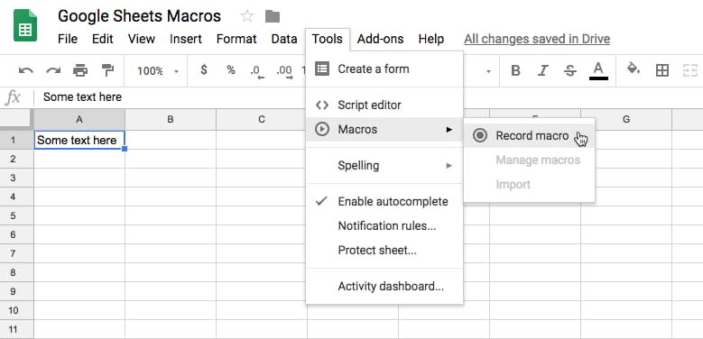
2) Go to the macro menu: Tools > Macros > Record macro
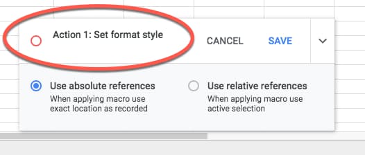
3) You have a choice between Absolute or Relative references. For this first example, let’s choose relative references:

Absolute references apply the formatting to the same range of cells each time (if you select A1:D10 for example, it’ll always apply the macro to these cells). It’s useful if you want to apply steps to a new batch of data each time, and it’s in the same range location each time.
Relative references apply the formatting based on where your cursor is (if you record your macro applied to cell A1, but then re-run the macro when you’ve selected cell D5, the macro steps will be applied to D5 now). It’s useful for things like formulas that you want to apply to different cells.
4) Apply some formatting to the text in cell A1 (e.g. make it bold, make it bigger, change the color, etc.). You’ll notice the macro recorder logging each step:
5) When you’ve finished, click SAVE and give your Macro a name:
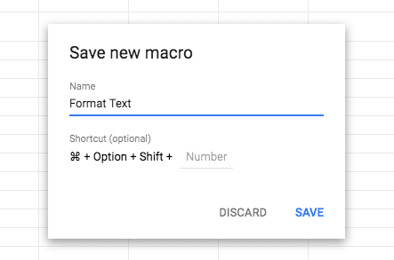
(You can also add a shortcut key to allow quick access to run your macro in the future.)
Click SAVE again and Google Sheets will save your macro.
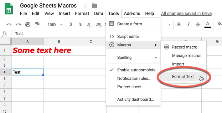
6) Your macro is now available to use and is accessed through the Tools > Macros menu:
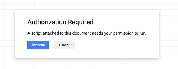
7) The first time you run the macro, you’ll be prompted to grant it permission to run. This is a security measure to ensure you’re happy to run the code in the background. Since you’ve created it, it’s safe to proceed.
First, you’ll click Continue on the Authorization popup:
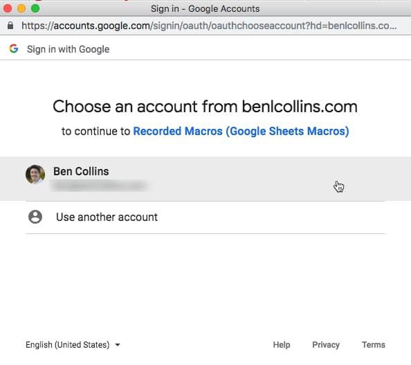
Then select your Google account:
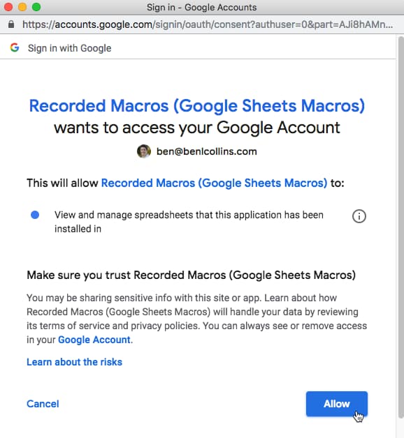
Finally, review the permissions, and click Allow:
8) The macro then runs and repeats the actions you recorded on the new cell you’ve selected!
You’ll see the following yellow status messages flash across the top of your Google Sheet:
![]()
![]()
and then you’ll see the result:
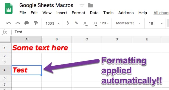
Woohoo!
Congratulations on your first Google Sheets macro! You see, it was easy!
Here’s a quick GIF showing the macro recording process in full:
And here’s what it looks like when you run it:
4. Other options
4.1 Macro Shortcuts
This is an optional feature when you save your macro in Google Sheets. They can also be added later via the Tools > Macros > Manage macros menu.
Shortcuts allow you to run your macros by pressing the specific combination of keys you’ve set, which saves you further time by not having to click through the menus.
Any macro shortcut keys must be unique and you’re limited to a maximum of 10 macro shortcut keys per Google Sheet.
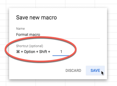
In the above example, I could run this macro by pressing:
⌘ + option + shift + 1
keys at the same time (takes practice ?). Will be a different key combo on PC/Chromebooks.
4.2 Deleting macros
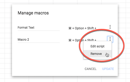
You can remove Google Sheets macros from your Sheet through the manage macros menu: Tools > Macros > Manage macros
Under the list of your macros, find the one you want to delete. Click the three vertical dots on right side of macro and then choose Remove macro:
4.3 Importing other macros
Lastly, you can add any functions you’ve created in your Apps Script file to the Macro menu, so you can run them without having to go to the script editor window. This is a more advanced option for users who are more comfortable with writing Apps Script code.
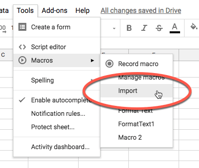
This option is only available if you have functions in your Apps Script file that are not already in the macro menu. Otherwise it will be greyed out.
5. Best Practices for Google Sheets Macros
Use the minimum number of actions you can when you record your macros to keep them as performant as possible.
For macros that make changes to a single cell, you can apply those same changes to a range of cells by highlighting the range first and then running the macro. So it’s often not necessary to highlight entire ranges when you’re recording your macros.
6. Limitations of Google Sheets Macros
Macros are bound to the Google Sheet in which they’re created and can’t be used outside of that Sheet. Similarly, macros written in standalone Apps Script files are simply ignored.
Macros are not available for other Google Workspace tools like Google Docs, Slides, etc. (At least, not yet.)
You can’t distribute macros as libraries or define them in Sheets Add-ons. I hope the distribution of macros is improved in the future, so you can create a catalog of macros that is available across any Sheets in your Drive folder.
7. A peek under the hood of Google Sheets Macros
Behind the scenes, macros in Google Sheets converts your actions into Apps Script code, which is just a version of Javascript run in the Google Cloud.
If you’re new to Apps Script, you may want to check out my Google Apps Script: A Beginner’s Guide.
If you want to take a look at this code, you can see it by opening the script editor (Tools > Script editor or Tools > Macros > Manage macros).
You’ll see an Apps Script file with code similar to this:
/** @OnlyCurrentDoc */

function FormatText() {
  var spreadsheet = SpreadsheetApp.getActive();
  spreadsheet.getActiveRangeList().setFontWeight('bold')
  .setFontStyle('italic')
  .setFontColor('#ff0000')
  .setFontSize(18)
  .setFontFamily('Montserrat');
};
Essentially, this code grabs the spreadsheet and then grabs the active range of cells I’ve selected.
The macro then makes this selection bold (line 5), italic (line 6), red (line 7, specified as a hex color), font size 18 (line 8), and finally changes the font family to Montserrat (line 9).
The video at the top of this page goes into a lot more detail about this Apps Script, what it means and how to modify it.
Macros in Google Sheets are a great first step into the world of Apps Script, so I’d encourage you to open up the editor for your different macros and check out what they look like.
(In case you’re wondering, the line /** @OnlyCurrentDoc */ ensures that the authorization procedure only asks for access to the current file where your macro lives.)
8. Examples of Google Sheets Macros
8.1 Formatting tables
Record the steps as you format your reporting tables, so that you can quickly apply those same formatting steps to other tables. You’ll want to use Relative references so that you can apply the formatting wherever your table range is (if you used absolute then it will always apply the formatting to the same range of cells).
Check out the video at the top of the page to see this example in detail, including how to modify the Apps Script code to adjust for different sized tables.
8.2 Creating charts
If you find yourself creating the same chart over and over, say for new datasets each week, then maybe it’s time to encapsulate that in a macro.
Record your steps as you create the chart your first time so you have it for future use.
The video at the top of the page shows an example in detail.
The following macros are intended to be copied into your Script Editor and then imported to the macro menu and run from there.
8.3 Convert all formulas to values on current Sheet
Open your script editor (Tools > Script editor). Copy and paste the following code onto a new line:
// convert all formulas to values in the active sheet
function formulasToValuesActiveSheet() {
  var sheet = SpreadsheetApp.getActiveSheet();
  var range = sheet.getDataRange();
  range.copyValuesToRange(sheet, 1, range.getLastColumn(), 1, range.getLastRow());
};
Back in your Google Sheet, use the Macro Import option to import this function as a macro.
When you run it, it will convert any formulas in the current sheet to values.
8.4 Convert all formulas to values in entire Google Sheet
Open your script editor (Tools > Script editor). Copy and paste the following code onto a new line:
// convert all formulas to values in every sheet of the Google Sheet
function formulasToValuesGlobal() {
  var sheets = SpreadsheetApp.getActiveSpreadsheet().getSheets();
  sheets.forEach(function(sheet) {
    var range = sheet.getDataRange();
    range.copyValuesToRange(sheet, 1, range.getLastColumn(), 1, range.getLastRow());
  });
};
Back in your Google Sheet, use the Macro Import option to import this function as a macro.
When you run it, it will convert all the formulas in every sheet of your Google Sheet into values.
8.5 Sort all your sheets in a Google Sheet alphabetically
Open your script editor (Tools > Script editor). Copy and paste the following code onto a new line:
// sort sheets alphabetically
function sortSheets() {
  var spreadsheet = SpreadsheetApp.getActiveSpreadsheet();
  var sheets = spreadsheet.getSheets();
  var sheetNames = [];
  sheets.forEach(function(sheet,i) {
    sheetNames.push(sheet.getName());
  });
  sheetNames.sort().forEach(function(sheet,i) {
    spreadsheet.getSheetByName(sheet).activate();
    spreadsheet.moveActiveSheet(i + 1);
  });
};
Back in your Google Sheet, use the Macro Import option to import this function as a macro.
When you run it, it will sort all your sheets in a Google Sheet alphabetically.
8.6 Unhide all rows and columns in the current Sheet
Open your script editor (Tools > Script editor). Copy and paste the following code onto a new line:
// unhide all rows and columns in current Sheet data range
function unhideRowsColumnsActiveSheet() {
  var sheet = SpreadsheetApp.getActiveSheet();
  var range = sheet.getDataRange();
  sheet.unhideRow(range);
  sheet.unhideColumn(range);
}
Back in your Google Sheet, use the Macro Import option to import this function as a macro.
When you run it, it will unhide any hidden rows and columns within the data range. (If you have hidden rows/columns outside of the data range, they will not be affected.)
8.7 Unhide all rows and columns in entire Google Sheet
Open your script editor (Tools > Script editor). Copy and paste the following code onto a new line:
// unhide all rows and columns in data ranges of entire Google Sheet
function unhideRowsColumnsGlobal() {
  var sheets = SpreadsheetApp.getActiveSpreadsheet().getSheets();
  sheets.forEach(function(sheet) {
    var range = sheet.getDataRange();
    sheet.unhideRow(range);
    sheet.unhideColumn(range);
  });
};
Back in your Google Sheet, use the Macro Import option to import this function as a macro.
When you run it, it will unhide any hidden rows and columns within the data range in each sheet of your entire Google Sheet.
8.8 Set all Sheets to have a specific tab color
Open your script editor (Tools > Script editor). Copy and paste the following code onto a new line:
// set all Sheets tabs to red
function setTabColor() {
  var sheets = SpreadsheetApp.getActiveSpreadsheet().getSheets();
  sheets.forEach(function(sheet) {
    sheet.setTabColor("ff0000");
  });
};
Back in your Google Sheet, use the Macro Import option to import this function as a macro.
When you run it, it will set all of the tab colors to red.
Want a different color? Just change the hex code on line 5 to whatever you want, e.g. cornflower blue would be 6495ed
Use this handy guide to find the hex values you want.
8.9 Remove any tab coloring from all Sheets
Open your script editor (Tools > Script editor). Copy and paste the following code onto a new line:
// remove all Sheets tabs color
function resetTabColor() {
  var sheets = SpreadsheetApp.getActiveSpreadsheet().getSheets();
  sheets.forEach(function(sheet) {
    sheet.setTabColor(null);
  });
};
Back in your Google Sheet, use the Macro Import option to import this function as a macro.
When you run it, it will remove all of the tab colors from your Sheet (it sets them back to null, i.e. no value).
Here’s a GIF showing the tab colors being added and removed via Macros (check the bottom of the image):
8.10 Hide all sheets apart from the active one
Copy and paste this code into your script editor and import the function into your Macro menu:
function hideAllSheetsExceptActive() {
  var sheets = SpreadsheetApp.getActiveSpreadsheet().getSheets();
  sheets.forEach(function(sheet) {
    if (sheet.getName() != SpreadsheetApp.getActiveSheet().getName())
      sheet.hideSheet();
  });
};
Running this macro will hide all the Sheets in your Google Sheet, except for the one you have selected (the active sheet).
8.11 Unhide all Sheets in your Sheet in one go
Open your script editor (Tools > Script editor). Copy and paste the following code onto a new line:
function unhideAllSheets() {
  var sheets = SpreadsheetApp.getActiveSpreadsheet().getSheets();
  sheets.forEach(function(sheet) {
    sheet.showSheet();
  });
};
Back in your Google Sheet, use the Macro Import option to import this function as a macro.
When you run it, it will show any hidden Sheets in your Sheet, to save you having to do it 1-by-1.
Here’s a GIF showing how the hide and unhide macros work:
You can see how Sheet6, the active Sheet, is the only one that isn’t hidden when the first macro is run.
8.12 Resetting Filters
Ok, saving the best to last, this is one of my favorite macros! 🙂
I use filters on my data tables all the time, and find it mildly annoying that there’s no way to clear all your filters in one go. You have to manually reset each filter in turn (time consuming, and sometimes hard to see which columns have filters when you have really big datasets) OR you can completely remove the filter and re-add from the menu.
Let’s create a macro in Google Sheets to do that! Then we can be super efficient by running it with a single menu click or even better, from a shortcut.
Open your script editor (Tools > Script editor). Copy and paste the following code onto a new line:
// reset all filters for a data range on current Sheet
function resetFilter() {
  var sheet = SpreadsheetApp.getActiveSheet();
  var range = sheet.getDataRange();
  range.getFilter().remove();
  range.createFilter();
}
Back in your Google Sheet, use the Macro Import option to import this function as a macro.
When you run it, it will remove and then re-add filters to your data range in one go.
Here’s a GIF showing the problem and macro solution:
9. Resources
If you’re interested in taking things further, check out the following resources for getting started with Apps Script:
💡 Learn moreLearn how to write Apps Script and turbocharge your Google Workspace experience with the new Beginner Apps Script courseMacro reference guide in Google Docs help
Macro reference guide in the Google Developer documentation
And if you want to really start digging into the Apps Script code, you’ll want to bookmark the Google documentation for the Spreadsheet Service.
Finally, all of this macro code is available here on GitHub.
Thank you very much. 🙂
Is there a Marco for printing a range of Columns in google sheets?
Thank you for this sneak peak. I am looking forward to the entire course. If you don’t mind answering a question, I’d love to learn more.
1. Is there a way to employ a macro (or app script) on any google sheet? Right now I only know how to copy and paste the script into my new spreadsheet where I then have to authorize all over again. By the time I complete those tasks I might as well have just performed the task by hand.
Thanks again.
Great question, Jason!
Unfortunately there’s no easy way to utilize macros in different Google Sheets, except by copy-pasting them into the script editor.
Per this forum discussion, you maybe able to create a library, but you’d still have to create a script and load the library, so doesn’t really save any time. Also, at the bottom of this article, it suggests you can’t do this anyway.
Seems like this would be a killer feature though. FWIW, I’ll pass this idea on.
Cheers,
Ben
Not sure that this is solves your problem totally but my workaround for this is to create a template sheet with all the common macros installed and create a copy of this template every time you need to make a new sheet with your common macros. A new script sheet with your code will be generated at the same time as generating the new copied sheet and macros enabled immediately. Where his doesn’t help is if you have an old sheet you need to add the macros to.
Nice idea. Thanks for sharing, Doug!
I have the same question as Jason. Is there a way to save the macro so that it’ll be available to all sheets?
Hi Yee,
Great question — see my answer to Jason above.
Hopefully one day?!?
Ben
Hi Ben,
Thanks a lot for your beautifull articles. I’m so happy with it.
Thank you Ben, these are great tips..
I made a dashboard which consists of Sales and other Kpis which I update every week using Import range formula. Is there a code I can use that as once I get the raw data in the dashboard is updated automatically?
Thank you, Ben. Great and useful examples.
I’m looking forward to see your Apps Script Blastoff! course. I suppose some VBA background wouldn’t hurt, is it?
I wish you all the good in the world for any of your courses.
Thanks, Celia! Coming soon… 😉
HI Ben,
i have a requirement • Let’s assume we have 5 columns A,B,C,D,E in google sheet
• there are 20 records with some values in each cell/column
• The user should be able to select a few rows and click a “button or link” in google sheet (this is the trigger for that function X or business logic implementation)
• That function X or business logic implementation should be able to
o identify selected rows,
o compare values in specific columns A,B,D for all “selected” rows (e.g. check if A1=A2 and B1=B2 and D1=D3) and
o insert 1 row for unique combination into same google sheet at the specified location and
o concatenate values in other columns which did not match
o This output needs to be added in the same Google sheet (let’s say) at row 15.
e.g.
A B C D E
1 2 3 4 5
2 3 4 5 6
5 6 7 8 9
1 2 4 4 4
1 2 5 4 5
If row 1 to 4 is selected then output should be
A B C D E
1 2 3,4 4 5,4
2 3 4 5 6
5 6 7 8 9
If row 1 to 5 is selected then output should be
A B C D E
1 2 3,4,5 4 5,4
2 3 4 5 6
5 6 7 8 9
See if you can suggest any thing with this.. Thanks in advance
Hi Ben,
I have a spreadsheet with formula being populated on all columns, and I am setting it using formula to appear depending on the date of the year. Which means at any one time, a column will have data populated.
Is there a way I can edit the script for it to only convert the columns with data generated into values, while keeping the rest of the columns with data intact?
Thanks for this helpful article! I would love to use these but I can’t seem to get them to stick! After I hit save, they say they’ve saved but I’m unable to click Manage macros or import – https://monosnap.com/file/eyf0icBd0tPblnrmFxDS2VN2G8xgBT.
Any idea why? This is with a google business apps e-mail, not sure if that matters.
Thank You, I am happy to have found this as I was looking for a way to learn the App Script coding. I am new to this but I am quit interested in doing a little or more with Google Sheets instead of Excel.
Hi, I love google doc and sheets. I am teaching math to local children. I use sheets to make worksheets for homework. I have a question in this regard. Please help.
I am trying make a sheet filled with each cell, rand numbers of 3 digit without duplicate. How to go about?
Try this
https://www.ablebits.com/docs/google-sheets-generate-values/
Depending on when I run the macro, there might be a different number of rows in my sheet. What’s the trick only only selecting cells THAT CONTAIN DATA before performing a particular task in a macro (like formatting or copying)? Thanks
Found it watching your videos. THANKS.
Here’s the trick…
var range = sheet.getDataRange();
I am trying go move some custom macro’s from Excel to Google Sheets. These macros use commands like ‘Select Case’ and ‘UCase’ etc. What I’ve read says that changing the command to ‘VBA.UCase’ should work, but I get ‘ReferenceError: “VBA” is not defined’. What am I missing? Also, is there a list somewhere of the VBA macro command equivalents to the Google versions that I could just rewrite with?
Hi,
I have a question, we have 2 levels of approvals for leave requests in our organization. Is there a way to write a scrip..I am providing the process flow for better understanding
1. Employee can raise a request for leave which will go to the 1st level
2. 1st Level Manager can Approve / Reject the leave application
3. Approval / Rejection of 1st Level Manager will go to the 2nd Level Manage
4. He / She can take a decision based on that
Hi,
I am trying one scenario in Google Sheet.
Say for example, I have five sheets and What I want is:
Create Index in Sheet1 where list the name of all 4 sheets and their respective link to navigate, i.e. column1: list of names & column2: list of links. And click this link will navigate to respective sheet.
I am able to list the Names but not list.
Please suggest
This is so helpful! I am running into one problem that I hope you can help with. I have a master payouts sheet for a business. I also have numerous sheets where specific payouts are documented for each specific facet of the business (paying sales reps, closers, affiliates, etc.) I use the import range functions to bring all the payouts into the master sheet and use a filter to hide blank rows. One column in each sheet and the master sheet is a checkbox that is used to mark the transaction as paid or unpaid. How can I import the checkboxes from each sheet into the master sheet instead of having the true/false logic show up and without interrupting the importrange?
Thanks!
1.Sir I want to creat a save button as well as reset button on Google sheets . The save button which after saving send data to sheet or to another work book on Google sheets . After saving the working sheet close automatically.
And also a reset button .
I am trying to create a macro that runs automatically when a cell (in a specific column) with a data validation list has a state change from any of the options to “published”. At that point I want the row to change color. I can create a macro to do this, but the person would have to run the macro. I want the macro to happen automatically when someone makes the change to “published. Is there a way to do this? I was thinking I could use VBA script in Excel but not sure how to do this in Google Sheets. Thoughts?
Hi, thanks for sharing these, Ben!
I have a quick question, Is it possible, using macro, to delete sheets and then import excel file to current google sheet (add new sheet)?
Thanks
Hi Ben
I want to give edit rights to the user bust don’t want to provide make a copy rights.
Is it possible through Script?
Hi Ben,
Are you able to use macros to make comments and assign to a user?
Thank you,
Dave
Hello!
Complete newbie to Sheets and the use of macros – so bear with me!
I have a spreadsheet where I would like to export the data in a row to another pre-made sheet. Recorded a macro and it works fine the first time. If I go to select a different row from the same spreadsheet and use the same macro, the data from the previous selection is used in the macro, not the new row of data. Hopefully that makes sense. I tries changing from absolute reference to relative reference with no success.
Thanks in advance for any help!
Tom
Please how can I write an app script to send a reminder to my mobile phone for birthdays of members of my organization.
I will so appreciate it
Thank you
Hey ben, I am Ashish, in my google sheets i want to use macros in such a way that it copies B1:E2 and pastes values (Ctrl+Shift+V) in A1:D2. I want this to repeat every minute from morning 9 to afternoon 4pm. Please note that E1 cell =CONCATENATE(HOUR(NOW()),”:”,MINUTE(NOW()))
E2 cell =GOOGLEFINANCE(“AAPL”,”PRICE”)
Now you understand that im trying to create an intraday chart from the googlefinance live price shown (delay doesnt matter).
If i run the macro of {copies B1:E2 and pastes values (Ctrl+Shift+V) in A1:D2}, it shows this :
Error The coordinates of the source range are outside the dimensions of the sheet.
Can googlefinance function not be macro triggered.
But if I manually press Ctrl+Shift+Alt+1, that is macro shortcut, it works. but the trigger doesnt work.
Please help I am badly stuck. Your help would be heartily appreciated
Hi Ben- trying to create a macro in one google sheets document. Inside of the document there are several sheets. I want to make a macro to take information from one sheet and post on a different sheet.
Your #6. Limitations of Google Sheets Macros- says this isn’t possible:
Macros are bound to the Google Sheet in which they’re created and can’t be used outside of that Sheet. Similarly, macros written in standalone Apps Script files are simply ignored.
Is this still true? or am i able to get this to work?
I have a google sheet: I created functions using google script, and I am trying to read this data from an excel file, but it gives me “#NAME” for the columns that call the google script function, how can I fix this?
Ben,
There is no one in the world like you who can teach Google Sheet so passionately.
I am a big fan of Google sheet and have learnt everything to make the life easier from you.
Everytime I get your email and there is something new to learn.
I recommend everyone to learn these thing. Even if you don’t use it more, it give you structured thinking ability.
Cheers Neha
Je cherche à faire un envoi automatique, via une macro. Je m’explique : J’ai créé une feuille d’absence sous GOOGLE SHEET – JAVASCRIPT, j’aimerais créer un lien cliquable. Serait-ce possible que ce lien cliquable fasse office d’enveloppe dans laquelle je glisserais ma feuille d’absence. Merci pour votre aide !
Ben, you are the best!
i want to split the row into different two different rows but
i have data from row A to I & want to split the row q into two or three parts how can i use a macro for the same but row a to i will be same when row q is split
Bonjour,
J’aimerais envoyer ce tableau de façon hebdomadaire directement depuis google sheet !
Comment faire ?
Date de départ h:mn Date de retour h:mn
année mois jours heures
0 0 0 0:00
I want to print sheet by making print button on sheet. Is it possible?
pl. guide us
Hi Mukesh,
Unfortunately, this is not possible, as Apps Script has no way to connect with your local printer.
Cheers,
Ben
When I run this filter I get the following error: Cannot read property ‘remove’ of null. Do you know why that would be?
Hi Ben, has there been any updates to the macro limitations? I would like to create a global macro that is available to run in any new google sheet. It defeats the purpose of macros for me if I have to create a new one for each new google sheet. I would like to have a permanent addon or at least a way to import the macro into the new sheet.
Hi Ben,
Thanks so much for this, this has taught me a lot!
Hoping I can get some help here – if I was to use this code, but wanted to limit it to copy and paste values up to the 3rd last column, how would I implement that?
// convert all formulas to values in the active sheet
function formulasToValuesActiveSheet() {
var sheet = SpreadsheetApp.getActiveSheet();
var range = sheet.getDataRange();
range.copyValuesToRange(sheet, 1, range.getLastColumn(), 1, range.getLastRow());
};
Hello Ben,
I’ve a spreadsheet on google sheet where I use Importhtm to get the information from an excel spreadsheet published in htm and run a macro to update it and I have a trigger calling this macro with minute timer.
It always worked fine but it hasn’t updated for 3 days and there’s a message loading and with a text of “Error
Loading data…”
Do you have any idea what could be happening?
The macro I use is:
/** @OnlyCurrentDoc */
function test() {
var spreadsheet = SpreadsheetApp.getActive();
spreadsheet.getRange(‘A2’).activate();
spreadsheet.getActiveRangeList().clear({contentsOnly: true, skipFilteredRows: true});
spreadsheet.getCurrentCell().setFormula(‘=IMPORTHTML(“https://test.htm”;”table”;1)’);
spreadsheet.getRange(‘A3’).activate();
};
Hii Benl,
Thanks for sharing this useful information.
I have so far learnt a lot from peoples like you.
I want to Import my excel file (other than csv) in my google sheet but dont want my existing formulas and tabs to be deleted. Also I want and option that to select a specific sheet from my desktop file and replace it with my existing google sheet tab.
Is there a way to create a macro to import data (html, csv etc) that is located on your hard drive
Hey Ben, Thank you for the great info.
I have a requirement to copy the data from the ” Source” sheet to the ” Master” sheet, and while doing, I always want to increment the data in the Master sheet. With the macro, I can copy and paste, but how do I need copy to the immediate next row from the previous increment? Is there any trick to do that, or if you have any app script that would be a great help? I appreciate any help you can provide.
Hi Ben,
Great lesson!
How would you run a macro which runs using the time-driven trigger, and the macro should apply to 1 specific sheet out of many sheets?
So the macro runs automatically with no human touch but does so on the specified sheet only.
Thanks!!
Is it possible to run a macro by selecting a checkbox? So it would apply the macro to that particular row when the checkbox in that row is selected.
Thank you very much.