
In this post, we’re looking at the new, powerful Tables in Google Sheets.
We’ll start with the basic benefits and features of Tables. Then we’ll look at how you can work with data with Tables using the new Views feature. After that, we’ll look at how to use Tables with formulas and structured table references.
What are Tables in Google Sheets?
Tables are a new feature in Google Sheets. They make it quick and easy to apply formatting and structural rules to a plain range of data.
There are a lot of benefits to using Tables to work with data (see below). I’m excited to use Tables in my Sheets workflows, especially the new Group By views.
Why should you use Tables?
There are many benefits to using Tables, including:
- Quick and easy to apply formatting
- Header row is automatically locked at the top of the Table
- Nice selection of pre-built Table templates
- Nice selection of pre-built styles
- Super easy to add dropdowns or smart chips to columns
- Formulas automatically applied down whole column
- Formatting and calculations are applied automatically to new rows
- Super easy access to filter and group by views
- Some folks will love the Structured Table formula referencing
- Built-in data validation with the column datatypes
When should you not use Tables?
Like any spreadsheet technique, Tables won’t be the best choice for every situation:
- Tables might be confusing to people who are unfamiliar with them
- They introduce additional complexity and clutter to Sheets that you might not want
- The structured Table reference formulas can be confusing to the uninitiated
- They work best with uniform underlying data. If your data has blank rows, subtotals, etc. then Tables may not interpret it correctly
- It’s sometimes not possible to convert large, complex datasets into Tables
Tables Basics
Pre-Built Tables
Currently, when we open a new Google Sheet, we’re prompted to create a new Table with the Pre-Built Tables sidebar:
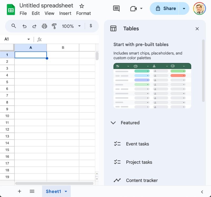
Using this, we can insert a pre-built table with a single click.
I doubt this will always open by default. It’s a deliberate choice to expose more people to Tables since they’re a new feature.
I see this being very helpful for people earlier in their Sheets journey. It showcases some of the best features — dropdowns, smart chips, etc. — that many folks don’t know about.
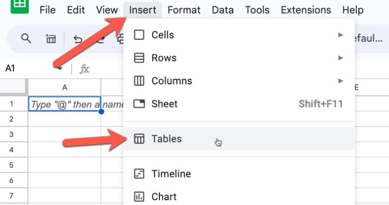
Access the Pre-Built Tables sidebar from the menu: Insert > Tables
How to create Tables in Google Sheets
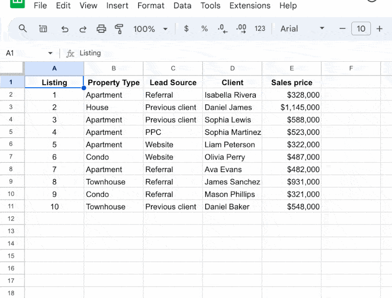
Now, suppose we already have this dataset in our Sheet:
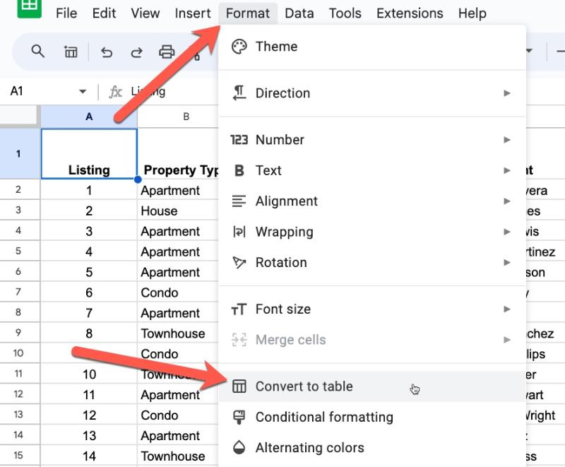
Click on any cell in a dataset and convert it to a Table via this menu:
Format > Convert to table
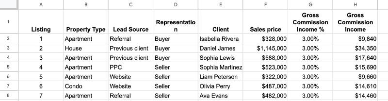
The new Table looks like this:
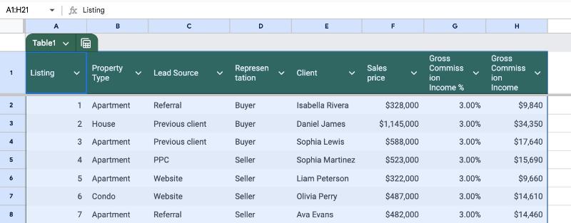
Now we can enjoy all the benefits of Tables that we mentioned above!
The main Table Menu
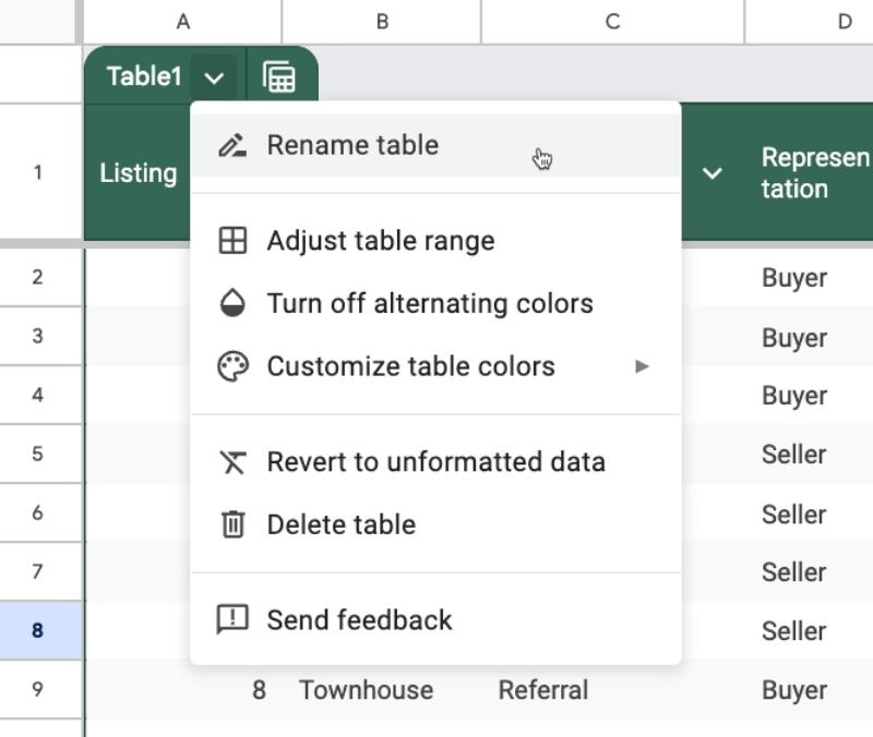
Click on the down arrow next to the Table name in the top left corner of the Table to open the Table menu.
From this menu, we can rename the Table, change the formatting, apply custom formats, or even delete the Table.
Be warned: Deleting the Table also deletes the underlying dataset. Use the “Revert to unformatted data” if you want to return to your base data.
The Column Menu
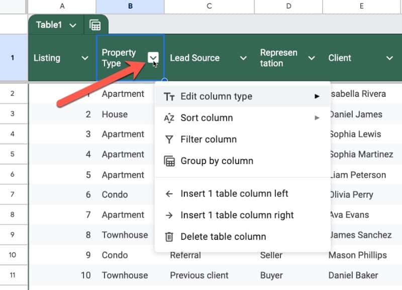
Click on the down arrow next to each column heading to open the Column Menu for that column.
Here, we can set the datatype for the column (i.e. is it text? A number? A smart chip?). This is a powerful setting so worth taking time to get to know.
For example, we can set a column to dropdown type and it will convert the entire column in a single click.
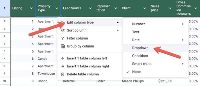
We can also filter and group by columns, which we discuss below.
And, there’s an easy way to add or remove columns from this column menu.
Data Analysis Tools Within Tables
One of the main benefits to using Tables with our datasets is the built-in data analysis tools that we get.
Built-in Data Validation
Setting column types can feel like an additional burden, but there are benefits.
One of the main benefits is the automatic data validation it provides.
Here’s how it works.
Suppose we set our column to be a Currency type column. This is shown by a small icon next to the column name (the first red arrow).
Then along comes a colleague who enters a new row. But they accidentally type a name (or other word) into that number column.
The Table will add a red warning flag and error message to indicate invalid data in that column:
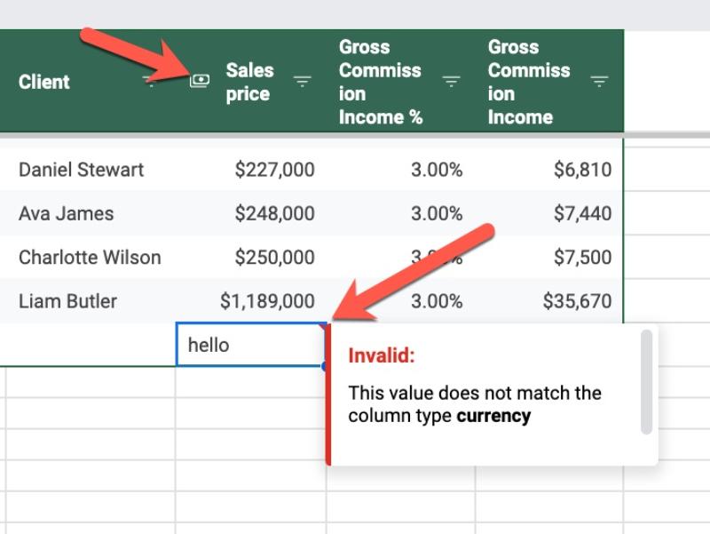
Table Views Menu
The Table Views menu is accessed from the Table icon next to the Table name, in the top left of the Table:
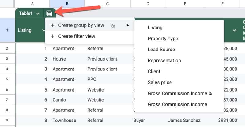
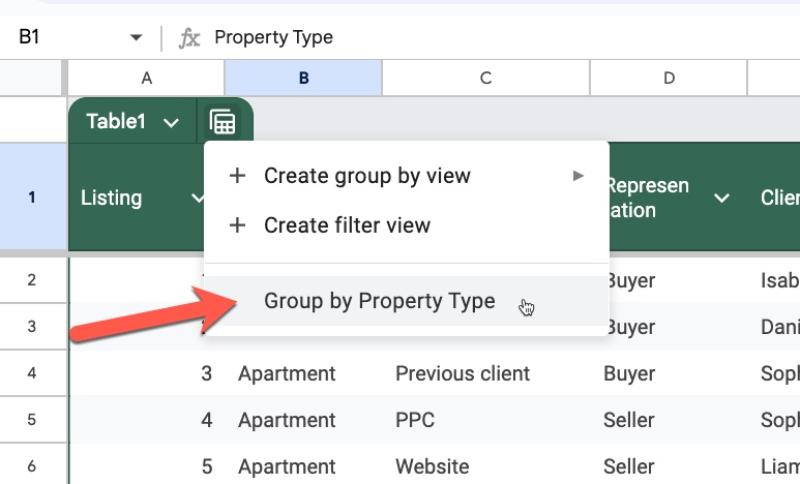
Opening the Table view menu lets us create Group By or Filter Views, or access previously built views.
Group By Views
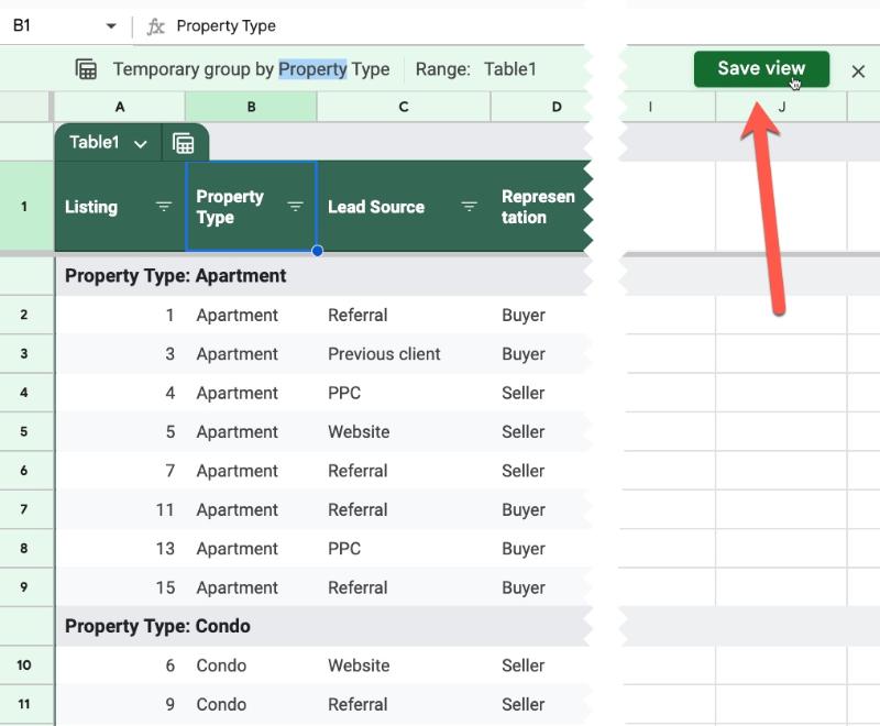
The new Group By View aggregates data into categories based on a selected column.
For example, we could group our data by property type with Group By View so that we can see all the groups together:
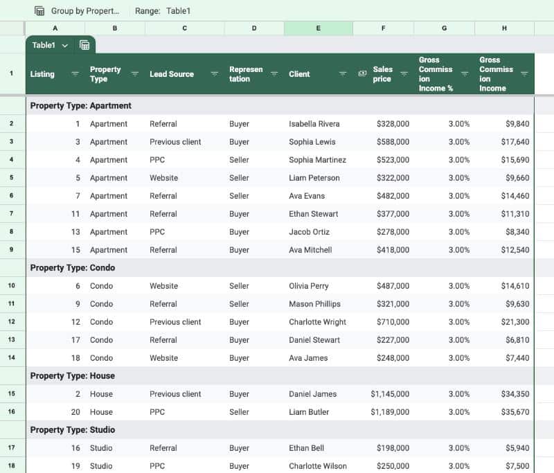
(One feature that is lacking with Group By Views is subtotal values for these groups. Fingers crossed we’ll get this in the future.)
Group By views can be created from either the Table View menu or from the selected Column menu.
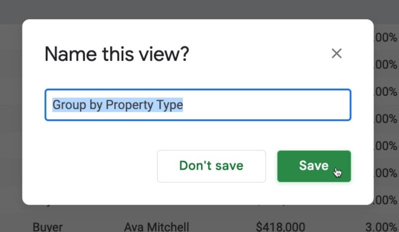
To save a View (Group By or Filter) click on the “Save view” button:
Give the view a name in the subsequent popup:
Now, this view will always be accessible from the main Table Views menu:
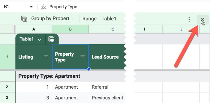
To close a view and return to the main Table view, press the “x” button on the right side of the green view bar between the formula bar and the Sheet.
Tables Filters
Filters are a HUGELY useful tool for exploring our data. They let us select subsets of data to review, based on categories (e.g. all the records for Client A) or conditions (e.g. all values over $100).
But many people aren’t aware they exist or forget to use them.
With Tables, they are applied automatically so that we can start using them immediately.
Access the Filter options inside the Column menu.
Tables Filter Views
Suppose we create a specific filter (all transactions with Client A over $100 in value) that we want to review over and over. Or share easily with colleagues.
We can create a Filter view and save this particular set of filter conditions to return to in the future.
Formulas In Tables
If you add a formula to the first row of a Table, you’re prompted to fill the entire column with Suggested Autofill:
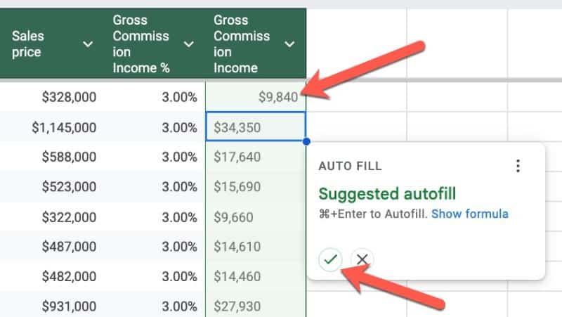
(Note: This is the same behavior as regular non-Table formatted data.)
Table Reference Syntax
Table References are a special way to access data inside a Table. Instead of A1-style cell references, we can use the Table name and Column headings in our formulas.
Let’s use this simple Table to illustrate the Table Referencing syntax:
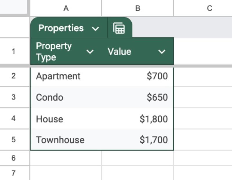
I’ve named this Table Properties.
(Note: Table names can only contain letters and numbers and can’t start with a digit or have a space.)
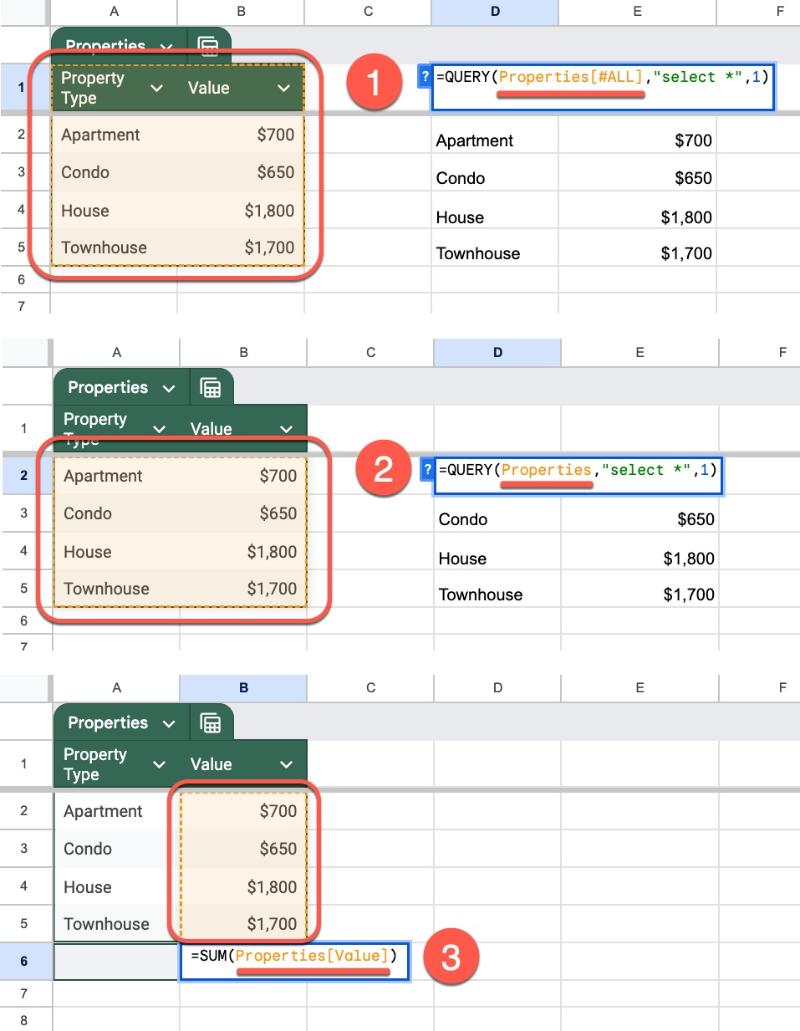
Here’s how the Table Referencing works:
Properties[#All]–> entire Table AND column headersProperties–> gets Table data only, NO column headersProperties[Column Name]–> gets data in named column only
(Note: column heading names CAN contain spaces, but must be unique within that Table.)
It’s easier to understand visually and I’ve added formulas to show how they work:
If you’re familiar with Named Ranges, then you’ll feel right at home using Table referencing.
(Note: you can still access cells inside Tables using regular cell references, e.g. =A1.)
Benefits of using Table References
There are a number of benefits to using Table References over standard A1-style cell references:
- The formulas automatically update to include any new rows of data added to the Table
- If you create, rename, insert, or delete columns in a Table, any Table References in formulas will automatically update too
- Easier to create than regular cell references. It’s easier to type “Properties[Value]” than e.g. “Sheet6!B2:B6”
- When you start typing a Table or Column name, the auto-complete box will show any Table References that you can quickly click
Using Table References in Formulas
Now we understand structured table references, let’s see them in action with a practical example.
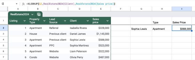
Let’s say we have a Table of real estate transactions. We call it RealEstate2024 (remember, no spaces allowed in Table names).
Now suppose we want to lookup a client name from that Table to retrieve transaction details.
To do that, we’ll use an XLOOKUP formula.
With our search term in cell G2 and using Table References, our formula is:
=XLOOKUP( G2 , RealEstate2024[Client] , RealEstate2024[Sales price] )RealEstate2024[Client] refers to the “Client” column inside the “RealEstate2024” Table. Similarly, RealEstate2024[Sales price] refers to the “Sales price” column inside that same table.
In our Sheet, it might look like this:
And here’s the equivalent A1-style formula:
=XLOOKUP( G2 , 'Copy of Sheet4'!D2:D21 , 'Copy of Sheet4'!E2:E21 )The Table Reference version is definitely cleaner and easier to understand.
Plus, any new rows of data added to the Table will be automatically included by the formula. Whereas, with the A1-style formula, we’ll need to remember to update the range references.
Now, I’m not about to tell you that you can throw away your A1-style referencing!
Tables References are super useful and worth using if you have your data in a Table. However, A1-style references are more flexible and still necessary for more complex formulas.
Hi Ben, great article as usual.
One question – are tables fully compatible with apps script do you know or are there considerations there we should be aware of?
D
Not yet. I hope that we get full support in the future though!
Ben, I am trying out tables but as you indicate that App script and tables are not compatible at the moment can one write a new script from scratch? My existing script return this sort of error Exception: You can’t apply a filter to a range that partially intersects a table. when I am using the same header rows and data set size!! I fear I may have to wait!!
Very nice.
But using QUERY, when I try selecting only some of the columns, I keep getting exception (no column Name) etc.
Can you please guide how to select some of the columns using Query in tables. Thanks.
With the QUERY function, it’s only possible to use A, B or Col1, Col2 etc.
Although you can write something like this:
=QUERY(Table1[#ALL],"select "&Table1[Data])it doesn’t give a meaningful output. It either gives a #VALUE! error or a repeating value if the QUERY formula is in the same row as the Table.
Cheers,
Ben
Hello Ben,
Yet another fine piece of work you have provided!!
I have the same questions as Danny and Ved.
I sooooo much want to be able to use table[column_name] in a QUERY function!! I have tried to do the ever popular “… ” & Table[colName] & “…” but it does not work.
Keep up the good work! You have helped me become a more powerful user of GSheets!!
Hi Michael,
Yes, unfortunately, it’s only possible to use A, B or Col1, Col2 etc.
Although you can write something like this:
=QUERY(Table1[#ALL],"select "&Table1[Data])it doesn’t give a meaningful output. It either gives a #VALUE! error or a repeating value if the QUERY formula is in the same row as the Table.
Cheers,
Ben
I would be curious to know your thoughts on the efficiency of using Structured Table referencing especially in using lookup functions like XLOOKUP. Generally I use the A2:A reference in a lot of my lookups, and I would think using the structured table reference would be more efficient when working with large sets of data.
Great question that I don’t have any hard data on yet. I would agree with you that the structured table references should be more efficient that open A2:A style references. Feel free to share any results here if run any experiments!
Hi!
If I used the filter Group by view, but I don’t want to keep it, How can I go back again?
The information moved to a table, but I’m not able to go back to the original format.
Thanks in advance.
Hi Ro,
Click on the table menu next to the table name and then select “Revert to unformatted data”.
Cheers,
Ben
Hi Ben,
It simplifies to use the Table column references when building formulas.
When I reuse my formulas in new tables, I would like to keep the column names intact inside the formulas. For example a reference like RealEstate2024[Sales price] in my formulas are changed to Sheet1!$E$2:$E$7.
What is a the quickest way to keep the simple names in the formula references intact when reusing a formula in another Table?
Do you also know if there is any script support of creating Tables?
Thanks for writing
Hi Ben,
first of all great work explaining this in such detail!
Do you know if it is possible to use a cell reference as a column name in a formula?
e.g. instead of =SUM(table1[Column_1]) I want to use =SUM(table1[“value in A1”]) where A1 contains the different column names in a dropdown (sales_aRet, sales_bRet, etc.). So far I wasn’t able to find a solution that works.
Keep up with your great work!
Best
Tobias
Is there no good way to reference the current row’s value in another column? In Excel, you would use Table[@Column], but I see no equivalent in Google Sheets.
Hi Andrew,
The syntax will only let you specify a column e.g. Table[@Column] as you guessed.
If you enter this as =Table[@Column] of a row that is part of that table, then it will grab the value from that specific row.
If you enter it elsewhere, not on a row that is shared with the table, you’ll see this error message “The default output of this reference is a single cell in the same row but a matching value could not be found. To get the values for the entire range use the ARRAYFORMULA function.”
Cheers,
Ben
Hi Ben,
I wanted my table to reference only the value in the same row within the table however it ends up getting the whole column for certain formulas i.e sum(filter). I have emailed you an image of the example. Is there a simple work around?
I have the same question and would love to have found the answer in this post.
I tried two things that seemed to yield suitable by-row formula evaluation in Sheets Tables, but failed (as of July 2025).
This in the first data row of the Table
=BYROW({MyTbl[Col01], MyTbl[Col03]}, LAMBDA(x, SUM(x)))
had the desired effect, at first – SUM by-row. BUT, when I used the built in ‘Insert Row Below’ plus sign button at the left of MyTbl, Sheets inserted a table-width row of cells below the first data row and copied all of formulas into this new row. The above =BYROW(…) could no longer expand, producing ‘#REF!’. The copy of =BYROW(…) in the new row expanded beyond the bottom of MyTbl. Failure
‘Using structured references with Excel Tables’ (https://support.microsoft.com/en-us/office/using-structured-references-with-excel-tables) describes
TblName[@[Col Name]]
as equivalent to
TblName[ [#This Row], [Col Name] ].
To replicate Excel’s ‘SUM(@[Col01], @[Col03])’ with Google Sheets, I entered
=SUM( MyTbl[ [#This Row], [Col01] ], MyTbl[ [#This Row], [Col03] ] into MyTbl[Col04]. The result in MyTbl[Col04] was correct! The Formula Bar showed =SUM( Sheet!$A2, Sheet!$C2 ). Google Sheets had correctly interpreted the structured references, but converted them to A1 form. Failure again.
A1 references for Table formulas for now. Google Sheet’s Table implementation lags well behind. I’ll stick to Named Ranges while awaiting progress.
“If you enter this as =Table[@Column] of a row that is part of that table, then it will grab the value from that specific row.”
That’s not what I found. Table[@Column], [@Column], or [@[Column]] are not understood by Google Sheets – returns a formula parsing error. Without the @ sign works fine.
Hi Ben,
When you change or format the column data to number >> currency, the default currency is in dollars $. How do we change this to other currencies?
Maybe try switching the location of the spreadsheet (File > Settings > General > Locale) and see if that helps?
Hi, Ben~
These new tables are awesome! Thank you for all the great info!
One thing I’m wondering that I haven’t figured out — is there a way to have “tags” within this new system?
I am a teacher working on a spreadsheet of info for all my students (name, ID number, parent/guardian contacts, home language, etc.) and one of the things I’d love to be able to see easily, and sort by, are programs a student is in, such as special education, language learner, talented and gifted, etc. I feel like I have seen table systems (maybe Awesome Table?) where I could pick which “tags” to associate with each student, so that I could look at one student/row and see what programs they belong in, but also use the new “views” feature to see the sub-set of students in each program.
Is something like that available with this new system? I can certainly use my old system of a set of columns for the special programs that are blank if they don’t apply, and check-boxed/’X’ed/otherwise labeled if they do apply, but just wondering.
Thank you!
Beth
Hey Ben, great article. Is it possible to save a ‘Table View’ as the default option when a spreadsheet is opened? I saved it as a view option that can be selected anytime but… I have a different tab for every month results. Created a Table View where I grouped everything by ‘Category’ then used that to make the relevant calculations….then realized every time I reopened the spreadsheet I had to go to each table and select the pre saved category view to get my calculations to work..
Hello! I am using a table in google docs for the first time today. Love this. But the only thing is that when I insert a new row, it is not keeping my formatting. There are no column borders on the new rows.
Hi Ben,
thanks for this detailed tutorial. I haven’t used tables yet, but thanks to your post I’ll give it a try. The local Micrsoft Office solution isn’t practical in the long run.
Hi Ben,
I often find your guides very helpful in puzzling out problems in Google Sheets, but I’ve *really* hit a stumper this time and I’ve been hitting nothing but dead-ends.
I’m playing around with these “new-fangled” Formatted Tables for a little personal project and I’m trying to make it a little bit “idiot-proof”… scratch that, “idiot-resistant”. The core setup involves a primary database in a separate sheet, which I maintain, that gets imported into a “Distribution Sheet” which people can make copies of and use for themselves. Each copy will pull its own instance of the Database (it’s small but periodically gets new lines added), processes the raw data, then displays it on a Formatted Table where Users can use a checkbox column to select which rows are “items” they possess. Then another part of the sheet will work with only the data for “items” they checked.
Now, as for the problem issue. Since there are currently over 50 “items” listed on the table, I wanted some filters available for Users to be able to quickly isolate “items” they’re interested according to categories of specific qualities. But I didn’t want them to have to fiddle around with the Filters directly. I set up a sort of “Dashboard” where they could use checkboxes and dropdowns to select or unselect options and those would serve as flags to control the filters. Then I’d implement Custom Formula filters into the Table which could automatically respond to the selections.
**But…** every time I try entering a Custom Formula for a Filter, the Address for where it references the “current row” it’s looking at keeps “shifting” somehow. For example, lets say I try the formula:
=ARRAYFORMULA(REGEXMATCH($E10,$E$8))
where E10 is the Header Line for my Table and E11 is the first data row for the Table. Also, E8 contains a String of, lets say for example, “colors” from that column constructed by using the join function with “|” as the delimiter: suppose I checked off red, green, and blue so it constructs a string “blue|green|red”.
Now, as I understand it, this *should* work similar to Conditional Color Formatting, except it starts with E11 instead of E10, and applies the “rule” by incrementing the row one by one in the Filter range; so E11> E12> E13> etc. And where it resolves to true, it keeps that row; where it resolves to false, it hides that row. But *instead*, what it seems to be doing is it’s *changing* the actual formula I put for the Custom Formula. After I Enter it, it hides **all** the Table rows, *only* showing the Header Row, and *also* it changes the Custom Formula from REGEXMATCH($E10,$E$8) to REGEXMATCH($E9,$E$8) all on its own. If I try entering it as REGEXMATCH($E11,$E$8), it won’t hide the rows of the table, but it also won’t respond to the checkbox controls and it also “steps back” the formula to REGEXMATCH($E10,$E$8).
This has happened with *numerous* other formulas I’ve attempted to use to address the issue, so I’m pretty sure it’s endemic to the Formatted Table system, itself. I need a way to directly refer to the data in the table, row-by-row, within my Custom Filter Formula in such a way that it can refer to the User-Set Dashboard Flags and *also* sort *all* the Data on the table, *including* the User-Selected checkboxes to indicate which rows they want to “Activate”. I know this was probably a lot, but for stuff like this I have a tendency to “overexplain to make sure I avoid underexplaining” #justautismthings
So, any suggestions?
Hi Ben,
Fantastic tutorial, thanks!
I have a bit of a pickle : if I use a query function to populate a table, the table range doesn’t adapt to the number of lines returned by the query.
Is there a way to achieve this?
Thanks.
Ah! I noticed this the other day too. It’s unfortunate. Presently, I don’t think there’s anything you can do about it but I will pass the feedback along to the Sheets team.
Brutal! This was my curiousity, too.
I’m still addicted to tables (Excel/PowerQuery guy). So I’ll overcome this limitation with a Error Handling sheet that checks # rows in sheet column versus # rows in table column for my tables which are populated by array formulas.
I just came across the following “Table Reference Syntax” that seems to be undocumented. If anyone has some more information about this nested bracket notation, please let me know.
Syntax:
tableTest[[color]:[h]]
Example: https://docs.google.com/spreadsheets/d/1_rfEs70YlnfeUPcSWOXkSljrjC_HyPjUHCZA2xzjAVE/edit?gid=0#gid=0
= XLOOKUP($B$15, tableTest[name], tableTest[[color]:[h]])
It seems to be documented now, see:
https://support.google.com/docs/answer/15637642
You can use table references to refer to:
A Table column: Table1[Column 1]
Across single columns: Table1[[#ALL],[Column 1]]
—> Across multiple columns simultaneously: Table1[[#ALL],[Column 1]:[Column 3]]
Excellent Guides Ben. Easy to understand and implement. My first goto when using sheets.
Thanks, Bob!
Tables in Sheets are still faulty. When trying to convert data into a table, it doesn’t use the selected header for your header, but selects your data and uses that first row as the header, and if you have formulas in any of those cells, it throws an error. Is there some way around that problem, without having to recreate the data?
I believe that this occurs if you have alternating colours applied to your data before converting it to a table. Remove the alternating colours, and then do the convert to table, and it includes the header row, if you had it selected.
FYI, the Table Reference syntax specifically does NOT work within Named Function definitions.
Using a reference of the form TableName[ColumnName] inside the Formula Definition field gives a Parse error.
You can see for yourself by trying to define a trivial function of the formula “=TableName[ColumnName]”
They work fine in lambda functions.
I was able to get the following to work in a named formula using the workaround of INDEXing into the table. While tbl[#HEADERS] doesn’t yet work in Sheets named formulas, OFFSET of row 1 of a table does; the header is -1 row off of table row 1.
For example, I defined a named formula called ASSOC(tbl, r, c) as a way of implementing a 2D associative array; this allows you to return the table value at the intersection of a row value and a header value; in the table called “tbl”:
Row Labels | Col 1 | Col 2 |
Row 1 | A | B |
Row 2 | C | D |
calling named function ASSOC(tbl, “Row 2”, “Col 1”) returns “C”
=INDEX(
tbl,
MATCH(r, INDEX(tbl,,1), 0),
MATCH(c, OFFSET(INDEX(tbl, 1, ), -1, 0), 0)
)
yes, I have used the offset location of the headers row inside Named Functions, myself, but my point is that the basic symbols themselves aren’t even resolved. Even the table name by itself (with no qualifiers) will resolve inside the Named Function
It would be nice if it temporarily omitted a grouped column from the table, to avoid needless repetition (Condo, Condo, Condo, Condo, Apartment, Apartment, Apartment, Apartment etc.).
Hiding it isn’t a viable workaround, as it’s not stored in the view, and the column remains hidden when the view is switched off.
I like the grouping – but if I move to a different tab it reverts to ungrouped data. Is there any way to default to a grouping or at least remember what I had grouped before I went to another tab?
I have to reselect the Group view every time I leave and return to the tab.
when do you reckon it will allow for subgroups within a group?
I am a convert to Tables. I use the following to access the entire column in a table
={OptSettings[Schedule Times]}
Simple and easy to read.
Do you see any “gotcha” in this?