Tag: data

In this post, we’re looking at the new, powerful Tables in Google Sheets.

We’ll start with the basic benefits and features of Tables. Then we’ll look at how you can work with data with Tables using the new Views feature. After that, we’ll look at how to use Tables with formulas and structured table references.

What are Tables in Google Sheets?

Tables are a new feature in Google Sheets. They make it quick and easy to apply formatting and structural rules to a plain range of data.

There are a lot of benefits to using Tables to work with data (see below). I’m excited to use Tables in my Sheets workflows, especially the new Group By views.

Why should you use Tables?

There are many benefits to using Tables, including:

• Quick and easy to apply formatting
• Header row is automatically locked at the top of the Table
• Nice selection of pre-built Table templates
• Nice selection of pre-built styles
• Super easy to add dropdowns or smart chips to columns
• Formulas automatically applied down whole column
• Formatting and calculations are applied automatically to new rows
• Super easy access to filter and group by views
• Some folks will love the Structured Table formula referencing
• Built-in data validation with the column datatypes

When should you not use Tables?

Like any spreadsheet technique, Tables won’t be the best choice for every situation:

• Tables might be confusing to people who are unfamiliar with them
• They introduce additional complexity and clutter to Sheets that you might not want
• The structured Table reference formulas can be confusing to the uninitiated
• They work best with uniform underlying data. If your data has blank rows, subtotals, etc. then Tables may not interpret it correctly
• It’s sometimes not possible to convert large, complex datasets into Tables

Tables Basics

Pre-Built Tables

Currently, when we open a new Google Sheet, we’re prompted to create a new Table with the Pre-Built Tables sidebar:

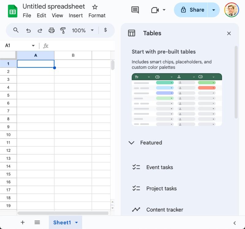
Using this, we can insert a pre-built table with a single click.

I doubt this will always open by default. It’s a deliberate choice to expose more people to Tables since they’re a new feature.

I see this being very helpful for people earlier in their Sheets journey. It showcases some of the best features — dropdowns, smart chips, etc. — that many folks don’t know about.

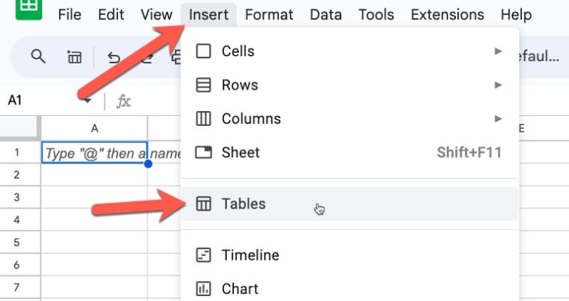
Access the Pre-Built Tables sidebar from the menu: Insert > Tables

How to create Tables in Google Sheets

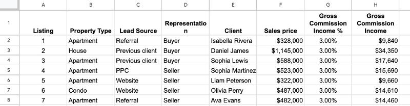
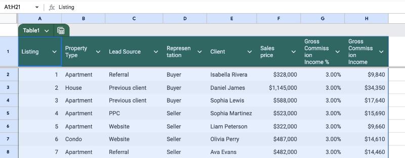
Now, suppose we already have this dataset in our Sheet:

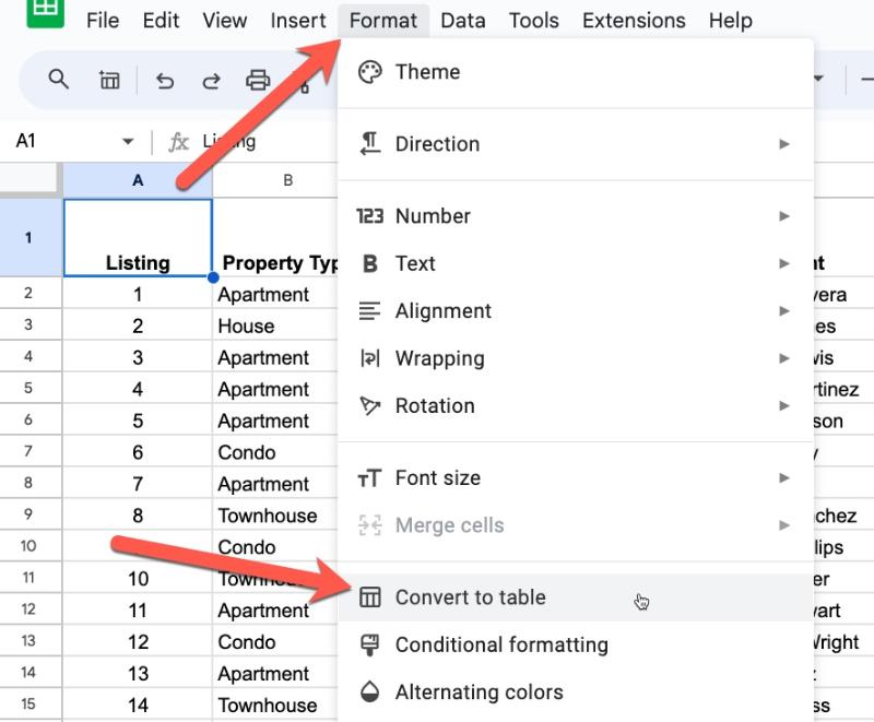
Click on any cell in a dataset and convert it to a Table via this menu:

Format > Convert to table

The new Table looks like this:

Now we can enjoy all the benefits of Tables that we mentioned above!

The main Table Menu

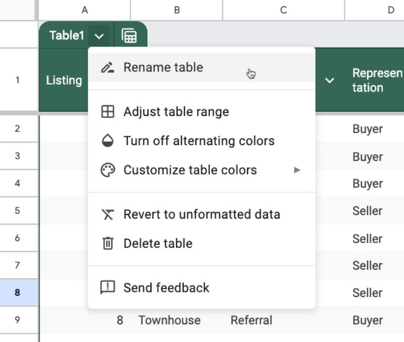
Click on the down arrow next to the Table name in the top left corner of the Table to open the Table menu.

From this menu, we can rename the Table, change the formatting, apply custom formats, or even delete the Table.

Be warned: Deleting the Table also deletes the underlying dataset. Use the “Revert to unformatted data” if you want to return to your base data.

The Column Menu

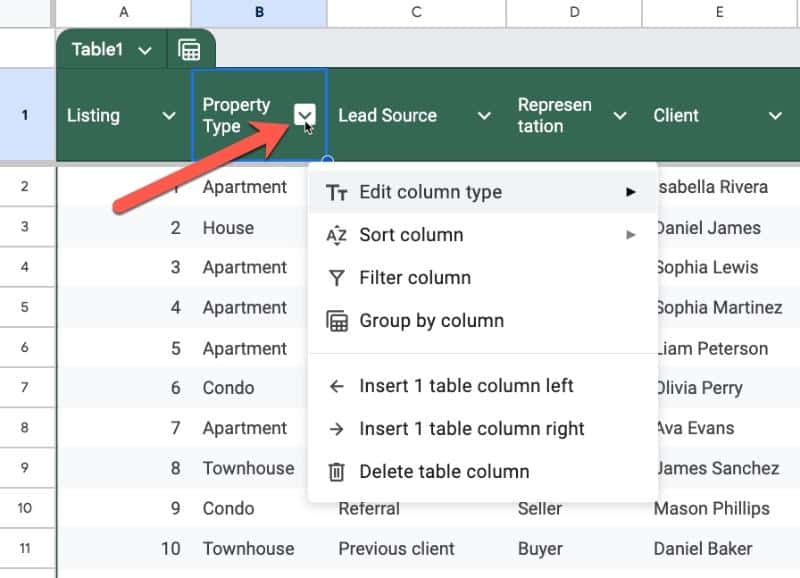
Click on the down arrow next to each column heading to open the Column Menu for that column.

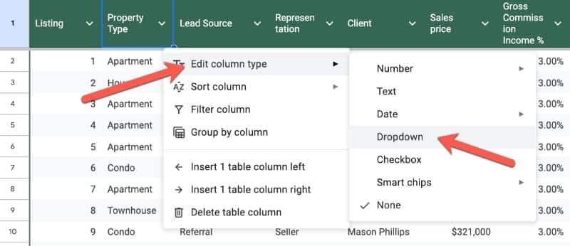
Here, we can set the datatype for the column (i.e. is it text? A number? A smart chip?). This is a powerful setting so worth taking time to get to know.

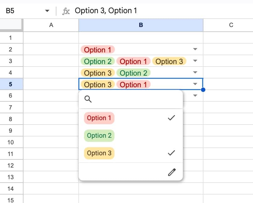
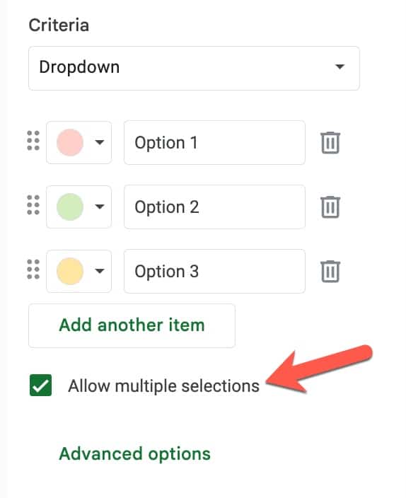
For example, we can set a column to dropdown type and it will convert the entire column in a single click.

We can also filter and group by columns, which we discuss below.

And, there’s an easy way to add or remove columns from this column menu.

Data Analysis Tools Within Tables

One of the main benefits to using Tables with our datasets is the built-in data analysis tools that we get.

Built-in Data Validation

Setting column types can feel like an additional burden, but there are benefits.

One of the main benefits is the automatic data validation it provides.

Here’s how it works.

Suppose we set our column to be a Currency type column. This is shown by a small icon next to the column name (the first red arrow).

Then along comes a colleague who enters a new row. But they accidentally type a name (or other word) into that number column.

The Table will add a red warning flag and error message to indicate invalid data in that column:

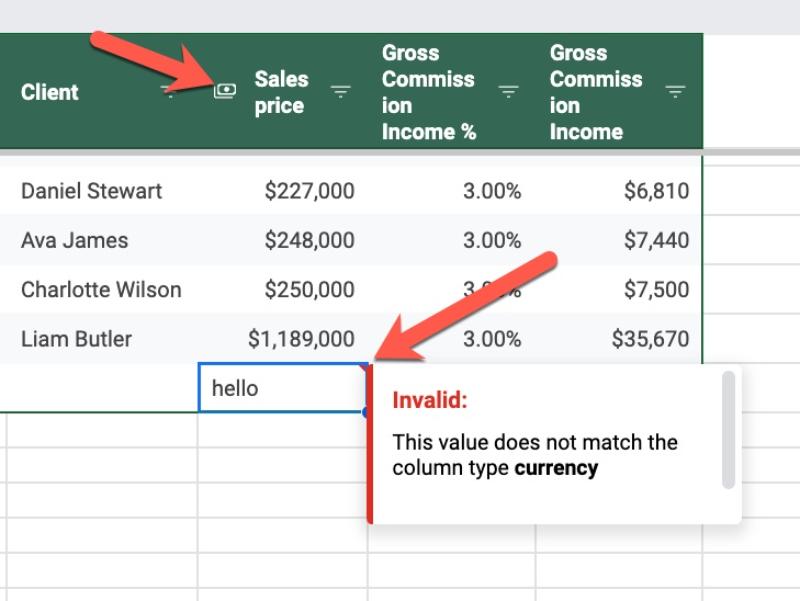
Table Views Menu

The Table Views menu is accessed from the Table icon next to the Table name, in the top left of the Table:

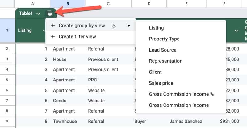
Opening the Table view menu lets us create Group By or Filter Views, or access previously built views.

Group By Views

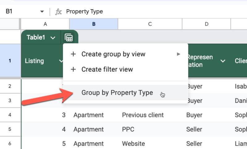
The new Group By View aggregates data into categories based on a selected column.

For example, we could group our data by property type with Group By View so that we can see all the groups together:

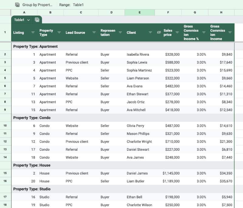
(One feature that is lacking with Group By Views is subtotal values for these groups. Fingers crossed we’ll get this in the future.)

Group By views can be created from either the Table View menu or from the selected Column menu.

To save a View (Group By or Filter) click on the “Save view” button:

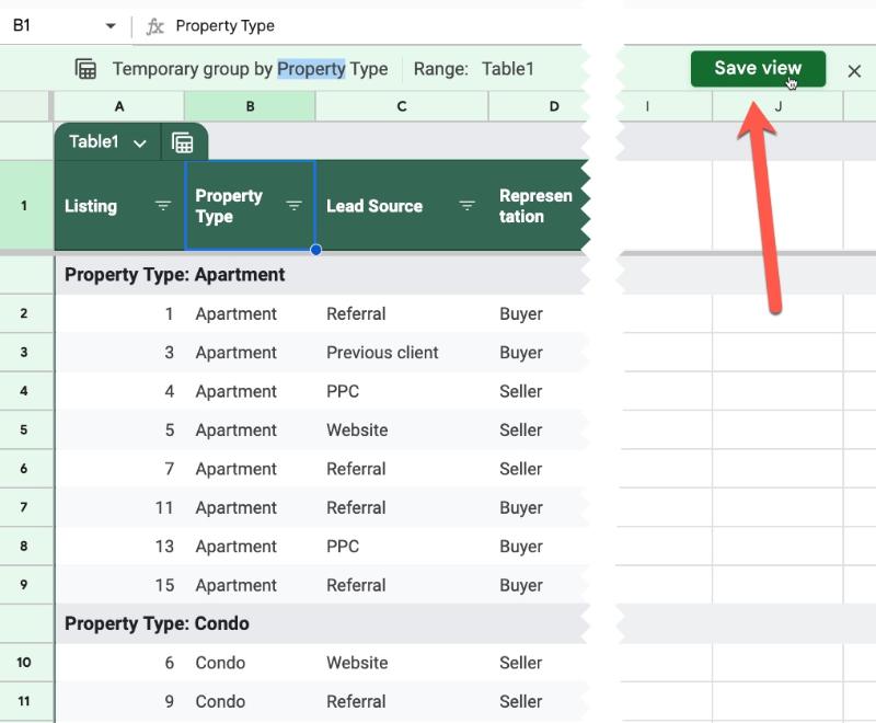
Give the view a name in the subsequent popup:

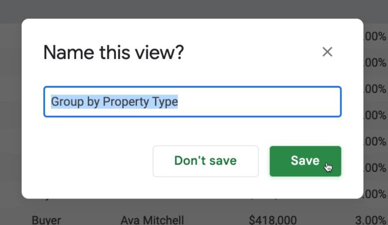
Now, this view will always be accessible from the main Table Views menu:

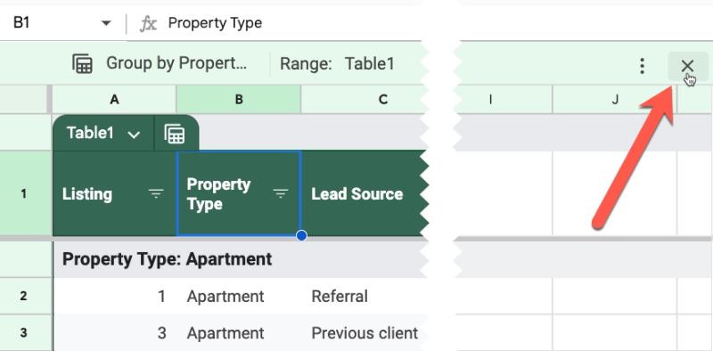
To close a view and return to the main Table view, press the “x” button on the right side of the green view bar between the formula bar and the Sheet.

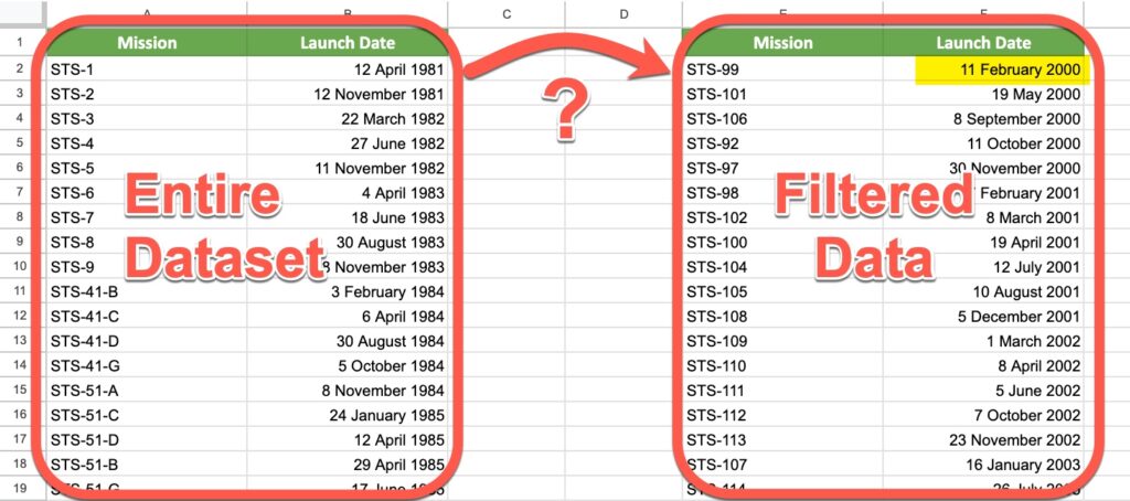
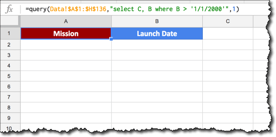
Tables Filters

Filters are a HUGELY useful tool for exploring our data. They let us select subsets of data to review, based on categories (e.g. all the records for Client A) or conditions (e.g. all values over $100).

But many people aren’t aware they exist or forget to use them.

With Tables, they are applied automatically so that we can start using them immediately.

Access the Filter options inside the Column menu.

Tables Filter Views

Suppose we create a specific filter (all transactions with Client A over $100 in value) that we want to review over and over. Or share easily with colleagues.

We can create a Filter view and save this particular set of filter conditions to return to in the future.

Formulas In Tables

If you add a formula to the first row of a Table, you’re prompted to fill the entire column with Suggested Autofill:

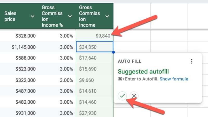
(Note: This is the same behavior as regular non-Table formatted data.)

Table Reference Syntax

Table References are a special way to access data inside a Table. Instead of A1-style cell references, we can use the Table name and Column headings in our formulas.

Let’s use this simple Table to illustrate the Table Referencing syntax:

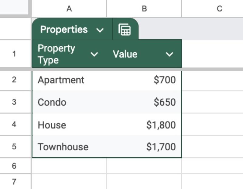
I’ve named this Table Properties.

(Note: Table names can only contain letters and numbers and can’t start with a digit or have a space.)

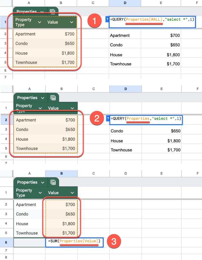
Here’s how the Table Referencing works:

1. Properties[#All] –> entire Table AND column headers
2. Properties –> gets Table data only, NO column headers
3. Properties[Column Name] –> gets data in named column only

(Note: column heading names CAN contain spaces, but must be unique within that Table.)

It’s easier to understand visually and I’ve added formulas to show how they work:

If you’re familiar with ​Named Ranges​, then you’ll feel right at home using Table referencing.

(Note: you can still access cells inside Tables using regular cell references, e.g. =A1.)

Benefits of using Table References

There are a number of benefits to using Table References over standard A1-style cell references:

• The formulas automatically update to include any new rows of data added to the Table
• If you create, rename, insert, or delete columns in a Table, any Table References in formulas will automatically update too
• Easier to create than regular cell references. It’s easier to type “Properties[Value]” than e.g. “Sheet6!B2:B6”
• When you start typing a Table or Column name, the auto-complete box will show any Table References that you can quickly click

Using Table References in Formulas

Now we understand structured table references, let’s see them in action with a practical example.

Let’s say we have a Table of real estate transactions. We call it RealEstate2024 (remember, no spaces allowed in Table names).

Now suppose we want to lookup a client name from that Table to retrieve transaction details.

To do that, we’ll use an ​XLOOKUP formula​.

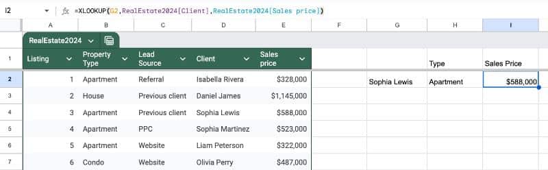
With our search term in cell G2 and using Table References, our formula is:

RealEstate2024[Client] refers to the “Client” column inside the “RealEstate2024” Table. Similarly, RealEstate2024[Sales price] refers to the “Sales price” column inside that same table.

In our Sheet, it might look like this:

And here’s the equivalent A1-style formula:

The Table Reference version is definitely cleaner and easier to understand.

Plus, any new rows of data added to the Table will be automatically included by the formula. Whereas, with the A1-style formula, we’ll need to remember to update the range references.

Now, I’m not about to tell you that you can throw away your A1-style referencing!

Tables References are super useful and worth using if you have your data in a Table. However, A1-style references are more flexible and still necessary for more complex formulas.

Further Resoures

Tables Documentation from Google