BYROW Function in Google Sheets – LAMBDA Helper Function

The BYROW function in Google Sheets operates on an array or range and returns a new column array, created by grouping each row to a single value.

The value for each row is obtained by applying a lambda function on that row.

For example, this BYROW function calculates the average score of all three rows in the input array:

Which looks like this in our Google Sheet:

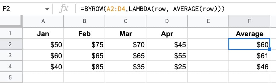
(Of course, you could use three separate AVERAGE functions to perform this calculation.)

But the important thing here is how the BYROW operates. It’s much more like programming.

We pass an array of data to the BYROW function.

It then passes each row into a lamba function to calculate a single value for that row (the average in this example). The BYROW formula returns these values in a column array, with the same number of rows as the original input array.

🔗 Get this example and others in the template at the bottom of this article.

BYROW Function Syntax

It takes two arguments:

array_or_range

This is the input array or range you want to group by rows.

lambda

This is the custom lamba function that is applied to each row. It must have exactly one name argument and one function expression. The name argument resolves to the current row.

BYROW Function Notes

The BYROW formula, given an input array with M rows and N columns, will return a column array with M rows and 1 column.

BYROW Function Example

BYROW can be used with the SPARKLINE formula to create a column of sparklines:

The output of this function is as follows:

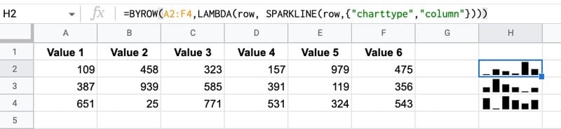
As with the previous average example, you could do this with the sparkline formula on its own, or even with an array formula version of the sparkline.

But it’s a different way of thinking with BYROW. You’re looping over the rows of data and passing the row into a function that operates on each row.

Using The BYROW Function With The FILTER Function

The BYROW function (and BYCOL function) work nicely with the FILTER function. It lets us perform calculations to use as filters without requiring a helper row.

We can set up the BYROW to return an array of TRUE/FALSE values, that we pass into the FILTER function as a filter condition.

Consider this dataset:

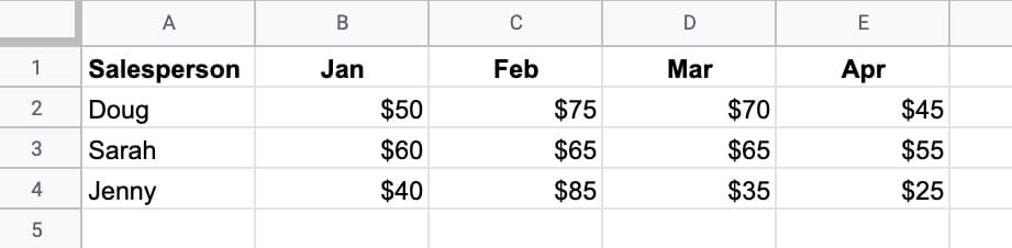
We want to filter on rows where the salesperson’s monthly average is greater than 50. Oh, and we’re not allowed to use a helper column.

Enter this BYROW formula as the first step:

Which creates an output array where each row is now grouped down to a single boolean value:

TRUE
TRUE
FALSE

(I.e. the rows for Doug and Sarah have averages > 50, but the row for Jenny does not.)

We can then pass this output into a regular FILTER function to display the names:

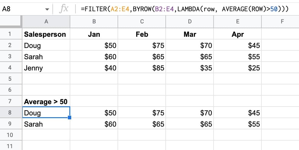
BYROW Function Template

Click here to open a view-only copy >>

Feel free to make a copy: File > Make a copy…

If you can’t access the template, it might be because of your organization’s Google Workspace settings.

In this case, right-click the link to open it in an Incognito window to view it.

See Also

See the LAMBDA function and other helper functions MAP, REDUCE, MAKEARRAY, etc. here:

Named Functions and New Functions In Google Sheets For 2022