Filtering with dates in the Query function in Google Sheets can be tricky.
In a nutshell, the problem occurs because dates in Google Sheets are actually stored as serial numbers, but the Query function requires a date as a string literal in the format yyyy-mm-dd, otherwise it can’t perform the comparison filter.
This post explores this issue in more detail and shows you how to filter with dates correctly in your Query formulas.
The Problem with Dates in the QUERY Function
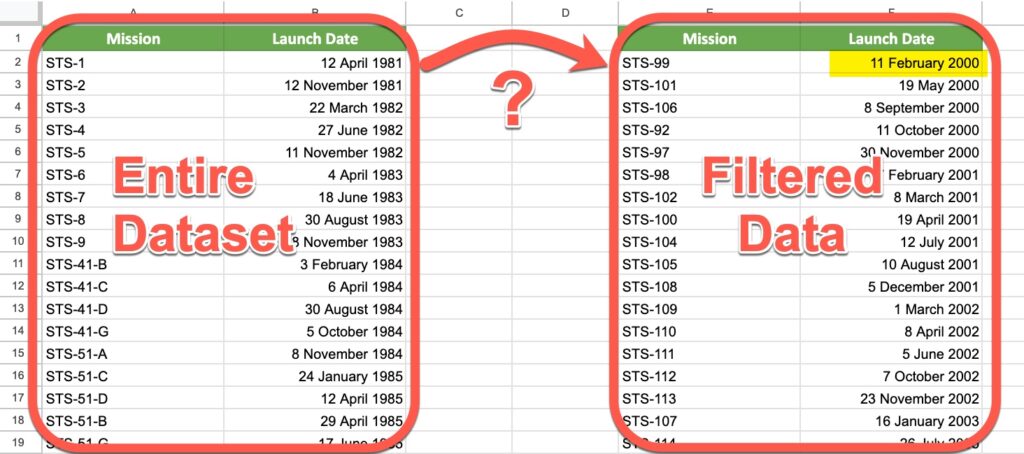
Suppose you have a dataset of Space Shuttle launches from the first launch in 1981 through to the final launch in 2011. You want to filter the data to look only at the subset from the year 2000 onwards.
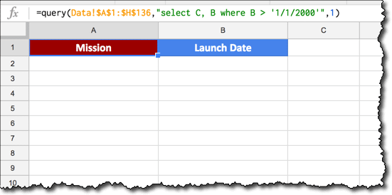
To begin, you might try the following syntax:
=QUERY(Data!$A$1:$H$136,"select C, B where B > '1/1/2000'",1)Unfortunately, the output of such a query is blank:
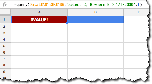
If instead we remove the single quotes from around the date and try again, we get a #VALUE! error because the Query formula can’t perform the comparison:
Alas, what are we to do!
Neither of these “standard” formats work, because the dates are not in the correct format for the Query function.
 💡 Learn more
Learn more about the QUERY Function in my comprehensive course: The QUERY Function in Google Sheets
Correct Syntax for Dates in the QUERY Function
Per the Query Language documentation, we need to include the date keyword and ensure that the date is in the format yyyy-mm-dd to use a date as a filter in the WHERE clause of our Query function.
Putting aside the Query function for a moment, let’s consider that "select..." string.
The new syntax we want will look like this:
date_column > date '2000-01-01'Our challenge is to create a text formula to create this syntax for us, inside our query function.
Dealing with the text function first, starting with our required date of 1/1/2000 and working outwards:
First, we convert it to a serial number format with the DATEVALUE() wrapper:
=DATEVALUE("1/1/2000")The output of this formula is a number:
36526Then the TEXT() function converts it to the required format for the Query formula by specifying a format of "yyyy-mm-dd":
=TEXT(DATEVALUE("1/1/2000"),"yyyy-mm-dd")The output of this formula is a date in the desired format:
2000-01-01Next we add single quotes around the new date format, with the "'" syntax. Finally, we insert the word date into the query string, to give:
="select C, B where B > date '"&TEXT(DATEVALUE("1/1/2000"),"yyyy-mm-dd")&"'"which gives or desired output:
select C, B where B > date '2000-01-01'That’s the syntax challenge done!
We can now plop that string into the middle argument of our Query function as per usual, and it’ll do the trick for us.
In this case, I was using a table of Space Shuttle mission data from Wikipedia, which contains a column of launch dates.
I used the IMPORTHTML() function to import that table into my Google Sheet, into a tab called Data in the range A1:H136. There’s a link to this dataset and worksheet at the end of the post.
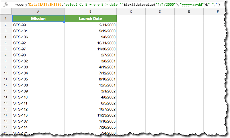
This Query formula returns all of the Space Shuttle missions after 1 January 2000:
=QUERY(Data!$A$1:$H$136,"select C, B where B > date '"&TEXT(DATEVALUE("1/1/2000"),"yyyy-mm-dd")&"'",1)The output of our formula is now returning the correct, filtered data:
Referencing a Date in a Cell
The formula is actually simpler in this case, as we don’t need the DATEVALUE function. Assuming we have a date in cell A1 that we want to use in our filter, then the formula becomes:
=QUERY(Data!$A$1:$H$136,"select C, B where B > date '"&TEXT(A1,"yyyy-mm-dd")&"'",1)Example Showing Filter Between Two Dates
Again, it’s relatively simple to extend our formula by adding a second date clause after the AND keyword:
=QUERY(Data!$A$1:$H$136,"select C, B where B >= date '"&TEXT(A1,"yyyy-mm-dd")&"' and B <= date '"&TEXT(B1,"yyyy-mm-dd")&"'",1)Today’s Date as a Filter
Substitute the TODAY() function into our formula:
=QUERY(Data!$A$1:$H$136,"select C, B where B > date '"&TEXT(TODAY(),"yyyy-mm-dd")&"'",1)Template
🔗 Click here to open a view-only copy >>
Feel free to make a copy: File > Make a copy…
If you can’t access the template, it might be because of your organization’s Google Workspace settings.
In this case, right-click the link to open it in an Incognito window to view it.
Thank you, great article as always
Is there an analogous method of summing durations (hh:nn) in queries? For me, sometimes the work when the original data is in hh:nn format. Sometimes I have to change them to a serial number for the query to work.
Yes, you can use the
timeofdayordatetimeliterals in the same way, although neither is exactly hh:mm format, so you’ll have to do some data manipulation too. They’re described in more detail here:https://developers.google.com/chart/interactive/docs/querylanguage#literals
How to solve the inter year problem solve. if we apply date condition with greater than date but date data show only upto 31 dec not show data after 31 dec from 01 jan
here is formula
=QUERY(IMPORTRANGE(“Link”,”FMS!A847:ab1000″),”Select Col28, Col2,Col1 where Col2 is not null and Col1>date ‘”&TEXT(DATEVALUE(“01/08/2023″),”yyyy-mm-dd”)&”‘”)
INSTEAD OF DOING FORMULA MORE COMPLEX GO WITH LITTLE SIMPLE LIKE:
=QUERY(IMPORTRANGE(“Link”,”FMS!A847:ab1000″),”Select Col28, Col2,Col1 where Col2 is not null and Col1>’2023-08-01′”)
Excelente gracias Ben
Dear Ben,
I have no words to thank you for your wonderful examples.
I did the spreadsheet with your “query” example and it worked for me. but I have a small problem:
The cell D1 is a list from an interval, there I choose the sellers ID (numeric), and in the formula I have:
AND
J = '' & D1 &and it does not bring me any results, I think because it’s numeric, I tried the following but it did not work:
AND
J = '"& TEXT (D1;" ########### ") &"'But it did not work 🙁
Please, can you help me? Thank you.
Hey Fernando,
Try it without any additional single quotation marks, like this:
J = " & D1If the datatype in cell D1 (number) matches the datatypes in column J (e.g. numbers as well) then it should work for you.
Cheers,
Ben
Hey Ben, you are amazing!
Thanks
Hey Ben, I have query here. Can we use the query formula in vlookup for range? the sheet I am referring to range has nearly 1 million records and I need to lookup for value based on Date Range, not in the whole data.
Dear Ben,
This year I have been creating a monthly summary of posts and updates associated with all things GSuite. It occurred to me after nine months that I should really be storing all the links in some sort of database. My question is how to automate the process of turning that into a monthly post (https://readwriterespond.com/2017/10/scripting-automated-solution/).
I have been getting on the GAS and am thinking that QUERY might be a part of my solution. I am therefore trying to get everything working in Sheets first. I have followed your guide to QUERY (https://www.benlcollins.com/spreadsheets/google-sheets-query-sql/), even adding in two dynamic selectors (is that what they are called?) that I got from your work on VLOOKUPS (https://www.benlcollins.com/spreadsheets/vlookup-wildcard/). My question is filtering by dates. I have followed your instructions, but fear that I maybe limited as I have recorded my dates using DD-MM-YYYY. Sheets recognises this as a date as a formatted the cells as ‘DATES’. My spreadsheet settings have also been changed to ‘Australia’. I am wondering if you have any thoughts or suggestions on this? Here is a link to my sheet – https://docs.google.com/spreadsheets/d/17Szdpgp3viqi2TsvYhF2Nfc97fQhWkhXQ-ZK9x9XQRM/edit#gid=1616853743&range=F2
Hey Aaron!
Cool project!
I made a copy of your sheet and changed the formula to this:
=query(gsuite, "Select F, G Where B = '"&A$2&"' and A = '"&B$2&"' and C > date '"&TEXT("2017/10/1","yyyy-mm-dd")&"' and C <= date '"&TEXT("2017/10/30","yyyy-mm-dd")&"'", 1)I made two changes: 1) put quotation marks around your start and end dates in the TEXT formulas; and 2) you had B instead of C in your last date comparison.
I think this query formula now works as you intended.
Cheers,
Ben
great help
i did:
=iferror(QUERY(order!A:AT;”select AK where AI= ‘”&B8&”‘ and Y >= date ‘”&TEXT(DATEVALUE(B14);”yyyy-mm-dd”)&”‘ and Y <= date '"&TEXT(DATEVALUE(B18);"yyyy-mm-dd")&"'";0);"0")
Bring the dinamic values between dates and a criterion
* where B8 is Data Validation
*and B14 and B18 are formated as date cell
* if value is empty in colum AK the result is 0
works fine
thanks
What is the alternate formula for “unique counta” with multiple criteria?
Hi Ben,
Thanks! You solved my problem!
But I got into another one… For some reason, it works fine when I have ” when Q > date ‘”&Text(F17, “yyyy-mm-dd”)&”‘ “, but the query is empty if I change the “>” sign for a “=” sign.
How can I filter my query so that it matches a specific date? (in your example, it would be for instance a list of shuttle missions on January 1st.
Thank you in advance.
Cédric
Hey Cédric,
Great question! We can use certain scalar functions inside of our query string to achieve this. Since there were no launches on 1 January, I’ve used 1 July instead and this formula to get back all data on the 1st July:
=query(Data!$A$1:$H$136,"select C, B where month(B) + 1 = 7 and day(B) = 1",1)Note, that if we wanted to get back data in the whole month of January, regardless of year, i.e. all shuttle flights that took off in January, then we could use this formula:
=query(Data!$A$1:$H$136,"select C, B where month(B) + 1 = 1",1)I’ve added both these examples to the end of the linked template Sheet.
You’ll also notice that I had to add 1 to the month(), that’s because it’s 0-based.
You can find more about these scalar functions here: https://developers.google.com/chart/interactive/docs/querylanguage#scalar_functions
Cheers!
Ben
Thank you Ben!
I used where Q > date ‘”&Text(A1-1;”yyyy-mm-dd”)&”‘ and Q < date '"&Text(A1+1;"yyyy-mm-dd")&"', but now I see that there is a more direct way of doing it. However, I would have to figure out how to reference a cell inside these scalar functions…
Hola Ben, en month(B) + 1 = 7, existe la forma de hacer referencia a una celda?, por ejemplo una lista donde esten todos los meses?
Hie Ben, thanks for expanding the formula.
How can i create a formula, where the same date has multiple entries, and i want the last entry of a specific date.
Hi Ben – You may not even respond to this BUT here’s to hoping! I am trying to show a person’s name from column D in a calendar-like Google sheet from another Google sheet with 6 columns. I followed your example above but it only returns the header row value (e.i., Name). I want to return the name of the person if one is returned ELSE NULL. Not sure what I’m doing wrong. Here is my code:
=IFNA(QUERY(Placements!A1:E1500, “SELECT D WHERE B>= date ‘ “&TEXT(DATEVALUE(“1/23/2023″),”yyyy-mm-dd”)&”‘ AND C<= date ' "&TEXT(DATEVALUE("1/27/2023"),"yyyy-mm-dd")&"'",1)," ")
/* 1 = header rows */
If I increase the value at the end to 2 or greater, it just concatenates all the values of that column up to that value. Example: Name Peter Monica Sally Nidhi, etc.
Hello,
I am trying to filter dates from last week and 3 week out from my spreadsheet. I keep putting the date function and still get an error. I was able to transfer by selecting A,B, C etc but now I just want those 4 weeks to show and when I put some new dates in the master spreadsheet I want it to automatically populate the query function spreadsheet. Can you help me with that?
I’ve searched far and wide to find a solution for TODAY() and always came up short until today. Thank you!
Hi Ben,
Please help me to get the totals by dates only from Date and time column in a query function.
See the sample below:
12/19/2017 11:15:58 23
12/19/2017 11:17:58 45
12/19/2017 12:10:58 56
12/20/2017 12:17:40 23
12/20/2017 12:17:40 67
12/20/2017 12:17:58 89
Result should be:
12/19/2017 124
12/20/2017 179
Thank you in advance.
Bijay
Hi Bijay,
Hope this will help you,
If you want to use dates and times, you need “datetime” instead of date. And since there is an interval, another comparison should be made with column B. The query string, shown with linebreaks for readability, would be
“select A
where B = datetime ‘” & text(A2, “yyyy-MM-dd hh:mm:ss”) & “‘”
This ensures that the datetime in A2 is between the datetimes in columns B and C.
Great!!!! Thx
Thanks a lot, was very helpfull 🙂
For I don’t know what reason, i had to change , to ; and columns letters to numbers so here is how the formula looks in my case :
={query({OOO!A2:AA1000;’Mauvais Contact’!A2:AA1000;’MER avec Contact’!A2:AA1000;’MER sans contact’!A2:AA1000};”select Col1, Col13, Col5, Col6, Col8, Col10, Col11, Col14, Col15 where Col13 > date ‘”&text(AM2;”yyyy-mm-dd”)&”‘ and Col13 date ‘”&text(AM2;”yyyy-mm-dd”)&”‘ and Col16 date ‘”&text(AM2;”yyyy-mm-dd”)&”‘ and Col19 date ‘”&text(AM2;”yyyy-mm-dd”)&”‘ and Col22 date ‘”&text(AM2;”yyyy-mm-dd”)&”‘ and Col25 <= date '"&text(AM1;"yyyy-mm-dd")&"'";1)}
Hi Sylvain,
Nice work! That’ll be because of your location. Sheets users in Europe use the ; notation instead of ,
See more under the Note subhead here: https://support.google.com/docs/answer/6208276?hl=en
Cheers,
Ben
Thnx, I tryed the examples but it did not work.
The , vs ; did the trick.
THnx
I am having difficulty in filtering date data Named Range ‘REPORTS’, for example cell
B1=Text(today(), "mm-dd-yyyy"), and if I want to count occurrences on this date with query like:=QUERY(REPORTS,"select COUNT(C) where B =date'"&text($B$1,"dd-mm-yyyy")&"' AND B='"&$A42&"'")But it works fine with > operator!
any thoughts
Hi Jas,
Is there a time component to the date in column B? That would be a reason why it doesn’t equal.
Maybe you could try two conditions, like this pseudo-code:
B1 >= today and B1 <= todayas a workaround? That should give you today only then...
Ben
Thanks! Very helpfull!
You’re welcome!
Thanks a ton! I’d been scouring stack overflow for how to do this. Super-helpful! 🙂
You’re welcome!
Could you please provide the syntax to do the same just for time also, and not date?
Thank you!
Hi Ben,
This is a great article, I have not used Query much before, let alone with dates, so this did help. This has got me half way to what I am trying to do and I was wondering if you could point me in the right direction?
I have a sheet listing items I need by date and use. Column A is the date (list the full year), then column F is the amount I need. I would like to look between a date range and just return the MAX number in F of that range only.
Could you give me any pointers?
Thank you
Alex
Hey Alex,
Have you tried something like this (using made up dates):
=query(data, "select max(F) where A < date '2018-02-01' and A >= date '2017-01-01' ", 1)This should calculate max F inside of your date range.
Cheers,
Ben
Hi Ben,
Thank you so much for this reply. I had the same issue 2 years later! One question. When I use this formula, it returns “max ColumnHeading” in the cell where I entered the formula, but spits out the result I want in the cell directly below it.
Is there something I can do so that it spits out the value I want in the cell where I entered the formula? I need to copy this formula to a series of rows, so everything has to be on the same line.
Should I be doing this with an entirely different function than query? Or will query do the job for me here? Thanks!
Hi again, Ben.
Nevermind; I answered my own question!
In order to get the value, I just turned the whole formula inside-out. That is, I put the MAX() function on the outside of the query.
(For context: my named range is “monthRange” and I’m looking for the highest value in column D out of all the rows where the year = 2020. )
Before (returns desired value in cell below):
=query(monthRange,”select MAX(D) where G=2020″,1)
After (returns desired value in same cell as formula): =max(query(monthRange,”select D where G=2020″,1))
I hope that’s helpful! Also, if you know of a better way to do it than this one, please let me know!
Thanks!
You saved the day!!! Thank you so much for your blog, this is the second time I’ve referenced it.
Thanks Denise!
Ran into this issue today and spent 30 mins trying to figure out why I wasn’t getting any results out. Glad I found this article, the solution is really well explained.
Thanks, glad it helped!
Hi Ben,
Long time reader. Love your site.
I ran into ONE issue with your “filter between two dates” formula. I am not sure if it was intentional.
I had a sheet where I was taking data that had multiple rows and values for the same date. You currently have it so that it will only sum the last occurrence for value of the date range. So:
Date Value
2018-04-01 1
2018-04-01 1
2018-04-02 1
2018-04-02 1
2018-04-03 1
With your formula, it would equal 4 instead of 5 because it would only count starting from the second 2018-04-01.
So the formula should read Where B >= date…. see below instead of just Where B > date…
=QUERY(Data!$A$1:$H$136,”select C, B where B >= date ‘”&TEXT(A1,”yyyy-mm-dd”)&”‘ and B <= date '"&TEXT(B1,"yyyy-mm-dd")&"'",1)
You have helped me so much, I thought I would return the favor by pointing something out. If this is intentional I would love to know why in case there is some huge flaw in this method. Thank you again for your help.
Hi Firdaush,
Thanks for your comment.
The “>” implies greater than, so it will count everything that is after that date. The “>=” is a greater than or equals to, so will include everything on that date as well.
Hope that helps!
Ben
Hi Ben,
I’m new to Google sheets. Thanks to Your website, it is very useful in my learning. I see there are lots of possibilities comparing dates with QUERY function. But, I’m trying to achieve this with the 2 sheets.
ResultSheet
I’d like to display the active employees in a for any given month.
MasterSheet
I have employees’ data in 3 columns, EmpName, DateOfJoin, DateOfReleive
Is this possible with QUERY function? Could you help me with this?
Thanks.
Here’s the file
https://docs.google.com/spreadsheets/d/1zd8yPYqOcdooFOUqcyj0v_XtW_hBPod3r_kK5maZkb0/edit?usp=drivesdk
Artigo Excelente. Muito Obrigado por compartilhar seu conhecimento conosco!
(Excellent Article. Thank you for sharing your knowledge with us!)
Thanks for sharing! It works perfectly
Hi There,
I Am Andres Felipe,
im working in a google sheet data base that i get from some google forms, im trying to filter the results of my query function by the timestamp of the responses but its not working.
=”Select C, X, O, Q, S, U, V Where ( D = ‘Acercamiento’ ) AND ( X >= date ‘ “&TEXT(DATEVALUE(A1),”yyyy-mm-dd”)&” ‘) Order by X desc format X ‘yyyy-mm-dd'”
this is the query formula i have so far.
thanks.
Hi Ben, I want ask you for advice. I want select some data (temperature) from column, but not by date as you show above, but by time. For example I’m interested in everyday temperature at 5. Could you please help me ?
Example datasheet: https://docs.google.com/spreadsheets/d/1RcdOaKci8zYCCOtb7y0h6yAcJgTrUuMfnjCVWYRXBy0/edit?usp=sharing
I try a lot, but it does’nt work. Thank a lot
Thank You Ben,
Great job.
Great Article. I am in need of some help with a workflow that I am creating where that references “today’s date” across multiple sheets and multiple columns where today’s date could be present. See example in the provided link.
https://drive.google.com/open?id=1weYkYevLrDP2xbxykWsHnlRmTtDXbKE5
There are possibilities for today’s date to be in columns K, M, N, O, or Q, which is consistent across four other sheets in this doc. Ultimately what I am trying to create is a daily task filter (which will be its own sheet) where my employee can follow up on sales leads that are in various stages of the sales process according to date.
Your help would be greatly appreciated. Thanks
Ben, great article. Is there a way to query multiple columns for the same date range? My sheet is hundreds of columns, and 5 columns are dates. I want to return rows where any of those 5 columns has a date within the desired range. Not all date columns have to fall within the range, just at least one. On top of that, it would be nice if it only returned an item once, even if multiple columns meet the date range.
Many thanks Ben, I’m finding this a great help in building a company time recording system.
Could you please advise me how to use query datetime from Google Forms something like this
=query(‘Sheet1’!$A$1:$B$100,”select A,B where A >= date ‘” & text(A1,”yyyy-mm-dd”) & “‘ and A < date '" & text(B1,"yyyy-mm-dd") & "'",1)
with A1 in Sheet2? This formula works with 1/1/2018 but not with 1/1/2018, 20:00:00. Thank you.
Interestingly enough, everything described above worked for me only once I removed the ‘date’ and left only something like:
A < '" & text(B1,"yyyy-mm-dd")
Ben, this is great stuff. I really appreciate it. What I’m trying to figure out is how to select based on the month. I want to be able to take a timestamp from a form entry, and then run the numbers from THIS month.
I was thinking that I could use something like, MONTH(TEXT(TODAY(),”yyyy-mm-dd”)), which would give me this month, and then search the log for months that match. But I’m no SQL expert here, and I’m not sure how to actually DO that.
Hi i was trying to filter out results if date column in worksheet1 lies within the range of date columns “from date” and “to date” in worksheet2 but getting error.
Below is my query:
=query(IMPORTRANGE(“14WxbiYeiY7fX6-V0f2MM4SraphCoa6EHD03F_6NmZ3g”,”Customer_Feedback_Report!A2:L250″),”select Col9 where Col8 = ‘”&Sheet1!A2&”‘ and Col4 > date ‘”&TEXT(‘”&Sheet1!J2&”‘,”yyyy-mm-dd”)&”‘ and Col4 <= date '"&TEXT('"&Sheet1!K2&"',"yyyy-mm-dd")&"' ",1)
it works if there is no date filter but with date filter it gives an error.
Col4 , j2 and k2 have datetype mm/dd/yyyy
hi BEN, I followed your exemples but my query with dates doesn’t work. Can you help me??
This is my query: QUERY(Consolida!$A$1:$L$4000;”SELECT B,C,D,E,F,G,H,L where D = date ‘”&TEXT(A2,”yyyy-mm-dd”)&”‘”,1)
It is in sheet called REPORT_TURRI IN A4 CELL and this is my spreadsheet:
https://docs.google.com/spreadsheets/d/1xADMqvsIModKaAFqctJ8Erv3J-ONaxCXUkxgLlvBB8I/edit#gid=2029169298
Thanks
Okay Ben –
Always hate to be the last question on a older thread, but here goes:
I am tracking direct reporting employees’ leave slips in google sheets so I always have the report view available via mobile device (and the intake forms as well)
Evaluating the data range for (in this instance) current day using your “today()” function inclusion for Query. Start Date and End Date are columns C & D, I am returning columns B & F (Name and Leave Type) for the report.
Using =QUERY(LeaveSlipFormIntake,”Select B, F WHERE date ‘”&TEXT(TODAY(),”yyyy-mm-dd”)&”‘ >= C AND date ‘”&TEXT(TODAY(),”yyyy-mm-dd”)&”‘ <= D", 1)
I am returning the correct fields but the wrong records (the evaluation is obviously occurring incorrectly). Is some of your prior examples you were performing scalar functions to manipulate the date against single cell references, can this be done against the column and if so how?
Thanks
Thanks for your help!!!
Hi,
I needed help on the following:
I wanted to filter by a date range – specifically any date that falls within the last year.
A B C
25 01/05/2018
25 01/07/2018
25 01/01/2016
C should say 50 as A1 and A2 fall within the last year.
This is the best idea i can think of at the moment:
=SUMIF(A:A,B:B,”>=today()-365)
But this didn’t work. Most of the above help is about extracting via query. I will be usinig query to get all the information i need to a second sheet and then wanted to filter by date.
Thanks is advance!
I’m trying to pass in the query from another cell – all works well until I start using dates – can you help?
https://docs.google.com/spreadsheets/d/1kxiJxH4vYX2iaqn0Toc0hMxdseRO-h_Ko55LiU8DXrs/edit#gid=0
See P9 and P10
Q10 works as desired – but I want to dynamically create the query string based on other conditions and thus being able to pass in the query string is a requirement (vs. parameterizing a literal string).
Thank you so much! This is exactly what I needed! The example sheet was super helpful, too!
Within a select statement I need to check the cell is an actual date.
So adding to a working counta… select… something like AND T = isDate()
Column T contains UTC date time and double numbers in a format of text as they are from an import
But this alway seems to return 0
Do you have an example of how to include an isDate test?
That is perfect. Thank you for the posting.
I am trying to use query to report counts for months My query string below does a good job but how do I get it to attach the year so it stays in chronological order instead of putting Jan at the top of my report.
=QUERY({Log!A2:T535},”select Month(Col1)+1,COUNT(Col3) group by Month(Col1) label Month(Col1)+1 ‘Month-Year’, COUNT(Col3) ‘Count'”)
Can you please give me some syntax to select a value from a date range? I have a spreadsheet for my fitbit and want to be able to select the total number of steps per month, based on date. the date column is column A, range is a5:a371. The steps are column B, b5:b371.
I changed the query to “=QUERY($A$5:$B$371,”select b where a > date ‘”&TEXT(A5,”2019-01-01”)&”‘ and a <= date '"&TEXT(B371,"2019-01-31")&"'",1)" but it is returning an error so obviously something is wrong.
I would also need a SUM function in there to add all of the January values together…
Thanks!
hi BEN, I followed your examples but my query with importing doesn’t work. Can you help me??
=QUERY(IMPORTRANGE(“14Uayi4V0usQVKal8px0qZYcCi9dcv53tHrxChGL_ZyY”,”data2!a3:e”),”select * where A = ” & A2 &””,1)
Dear Ben,
Thank you very much for your post. It’s illuminating as usual. Would it be possible for you to help me with my query problem?
I’ve been trying to fetch a specific date from Google Finance data using this syntax:
=QUERY(GOOGLEFINANCE(A2;”all”;TODAY()-52*5;TODAY());”select Col1 where Col3 >= (Q2)“;0)
A2 is the name of the stock, e.g. AMZN
Q2 is the cell containing the 52-week highest price.
All I’m trying to get is the date where the highest price was reached.
Other readers are also welcome to answer this question. Thank you in advance.
Sincerely,
Albard
Hola Ben, como hago referencia a una celda dentro de una función escalar?
Hi Ben,
I have a QUERY which doesn’t quite work and I have no idea why,
=query((TRANS.!A:G,”Select E,SUM(G) group by E,0),where A>DATE'”&B6&”‘and A<DATE'"&C6&"'))"))
B6 is reference start date e.g. 2019-01-02
C6 is a reference end date, e.g. 2019-12-31
and both reference at correct.
E a expense category for each individual data point which is supposed to sum in G.
I have both the data clause working separately as well as the expense category clause working separately. But they are not working together. Any help would be appreciated.
are there just extra quotes? And it looks like you might have backticks instead of single quotes in some spots.
Hi,
Is there any way to do the following:
The date, March 25, 2019, appears in column B and I want my formula to tell me when 2 weeks (or 10 business days) from that date is.
Great article Ben.
My experience is that date comparison is best handled by treating it as a number. If the date is to be constructed from year, month and date then DATE function may be used.
This operator like + and – can also be used to get dates few days early or late.
Regards
Hello there
Why I purpose change the date today data 4/3/3019 to MY A2 4/4/2019 9:28:53 the data in the query does not update i.e. disappear from the list?
Formula : =query($A$1:$B$25,”select A, B where B > date ‘”&text(TODAY(),”yyyy-mm-dd”)&”‘”,1)
Line Date
MY 2 4/3/2019 9:25:41
MY LAM 4/3/2019 9:27:14
MY 2 4/3/2019 9:28:05
MY LAM 4/3/2019 9:28:40
MY A2 4/3/2019 9:28:51
MY A2 4/4/2019 9:28:53
MY 2 4/3/2019 9:28:54
MY 2 4/3/2019 9:30:23
MY A2 4/3/2019 9:30:54
MY LAM 4/3/2019 9:31:07
MY 11 4/3/2019 9:31:27
MY LAM 4/3/2019 9:31:47
MY AS1 4/3/2019 9:32:37
Raw Data
Line Date
MY LAM 4/2/2019 21:20:40
MY A2 4/2/2019 21:19:40
MY A2 4/2/2019 21:19:51
MY 2 4/2/2019 21:21:35
MY 2 4/2/2019 21:23:48
MY A2 4/2/2019 21:26:24
MY LAM 4/2/2019 21:28:48
MY 2 4/2/2019 21:21:35
MY 2 4/2/2019 21:23:48
MY A2 4/2/2019 21:26:24
MY LAM 4/2/2019 21:28:48
MY 2 4/3/2019 9:25:41
MY LAM 4/3/2019 9:27:14
MY 2 4/3/2019 9:28:05
MY LAM 4/3/2019 9:28:40
MY A2 4/3/2019 9:28:51
MY A2 4/4/2019 9:28:53
MY 2 4/3/2019 9:28:54
MY 2 4/3/2019 9:30:23
MY A2 4/3/2019 9:30:54
MY LAM 4/3/2019 9:31:07
MY 11 4/3/2019 9:31:27
MY LAM 4/3/2019 9:31:47
MY AS1 4/3/2019 9:32:37
Great article!! Thank you.
I am trying to run a query to pull data from an based on the current month and the current year. However, it doesn’t work when I use the TODAY() function neither when I try to use the date from a populate cell (=TODAY()). It works only when I write the date (yyyy-MM-dd) which makes it not so ‘smart’ query anymore. Well
Query:
=query(Monthly_T!1:100000, “Select * Where month(A) = month(date’2019-04-10′) and year(A) = year(date’2019-04-10′)”,1)
I entered the Today date (=TODAY()) on cell A1 of the new sheet where the query is running and tried to replace the ‘2019-04-10’ but it didn’t work. Also entered ‘2019-04-10’ in another cell and tried to refer it in the query. it didn’t work either.
By the way, all dates are formatted as yyyy-mm-dd.
Any idea how to solve this?
ThankS!
I have the formulas below. The second works. If I take the SQL from the second formula and put it in cell B2, the first formula doesn’t work. Why is that? (it breaks with or without ” quotes, and with “””” in place of “). Is there some limit on the sql length?
1. query(Sales!A:AB,B2,1)
2. query(Sales!A:AB,”select A,B,C,D,G,K,L,M,N,O where K > date ‘”&TEXT(B1,”yyyy-MM-dd”)&”‘ and K < date '"&TEXT(C1,"yyyy-MM-dd")&"'",1)
I’m trying to Query a range of cells with dates in them in a DIFFERENT spreadsheet and Print the number of cells that meet a criteria (greater than or equal to a date in a cell in the CURRENT spreadsheet) into a cell. I’m having all sorts of issues. I even tried to just import the data and run a COUNTIF and that isn’t working.
to use a contemporary colloquialism :
This article was Too Legit to Quit
thanks for the assist!
I Ben,
I have the following scenario, a table filled daily with data, and an input cell where i write a date; I ‘d like to filter in order to show the rows date-2, date-1 and date.
Can you help me?
Cheers.
Beppe
Hey Ben!
Thanks So much for providing the right syntax!
I was struggling with it for past 2-3 days, but finally it worked with your inputs.
The following Query function now helps me fetch all that want from a data table:
=QUERY(rangeSourceData,”SELECT A,B,C,D,E,F,G where A > date ‘”&TEXT(rangeFromDate,”yyyy-mm-dd”)&”‘ and A < date '"&TEXT(rangeToDate+1,"yyyy-mm-dd")&"'",-1)
🙂
Hey Ben,
I have the function built out correctly but it wont pull in the data? Not sure if I am setting up my columns wrong or what. It pulls in the data headers but not the data itself.
=QUERY(‘Form Responses 2’!$A$1:$O$1078, A1,1)
Select * Where G = “Bark” AND A >= 43708
I can share the doc as well not sure what I am doing incorrectly.
Just looking to sort by date range and specific commodity.
Hi,
Can anyone help me with the query below? I get the error “Unable to parse query string for Function QUERY parameter 2: PARSE_ERROR: Encountered ” “7 “” at line 1, column 41. Was expecting one of: “group” … “pivot” … “order” … “skipping” … “limit” … “offset” … “label” … “format” … “options” … “and” … “or” …”
=QUERY($A$1:$G$136, “select C, B where B < date '"&TEXT(P3,"yyyy-mm-dd")&"' 7 offset "&(MAX(COUNT(B:B)-7)))
Hi Rashed,
Put comma before 7 offset & try again. If not resolved, share with me, I’ll rectify it
Hi Ben,
Your teaching is *almost* getting through my thick head. For the formula
=QUERY(Data!$A$1:$H$136,”select C, B where B > date ‘”&TEXT(A1,”yyyy-mm-dd”)&”‘”,1)
Why is
date ‘”&TEXT
correct instead of
date ‘&TEXT
That extra quotation mark is driving me batty
Hey Eric,
The extra quotation closes the first part of the string so you can use a function next (to generate the date dynamically) and then you need to use the close the string off again. The date also needs to be wrapped with single quotes, which is why you have to add a single quote to the string at the end. Just try playing with this formula to understand how it works:
="select C, B where B > date '"&TEXT(A1,"yyyy-mm-dd")&"'"Hope that helps!
Ben
Ahh … got it.
The coloring of the function confused me for a bit.
THANKS !
this is such a common use case… Why the F**k can’t they fix it to make it less terrible?
Does datediff() not work as advertised directly in the query formulas?
Dear Ben,
Thank you for your great help and time creating this valuable information!
I’m probably having a really light problem but one that I couldn’t figure out. I’d like to filter my data table by dates but my date column comes from a formula using a Timestamp(script). It goes like this: =if(G224 = “Paid”, timestamp(), ” “)
Basically, when I change G224 to “Paid” it gives me the current date in that cell. So, some cells in date column are empty and some are with the date.
After that I want to use query function to filter by date and i use this:
=query(myrange,”select A,B, C, I where I > date ‘”&text(B18,”yyyy-mm-dd”)&”‘”, 1)
in B18 I specify the date after which I want to get data.
“I” column is the column where I have timestamped dates. Timestamp date appears in format 31-10-2019. So, when I use it I get no result, no mistake but also no data pull. Might that be due to the fact that I have a formula for the date column? And if so, is there any way to work around it?
Thank you in advance!
Hello Ben,
Thanks for the article.
My question is: how to convert datetime (in format of string) to date inside a query?
What I have (string, without option to change format here):
2019-10-16 15:18:38
2019-10-16 18:02:23
2019-10-16 18:38:32
What I need (date format):
2019-10-16
2019-10-16
2019-10-16
I would prefer not to create additional columns in my dataset. Default format change is not an option. How to make this conversion via query?
Thanks in advance,
Nikita
Hi Nikita,
You can do this with the TEXT function embedded inside the QUERY function, it’ll be similar to the examples shown in this article.
Ben
how to Write Query having Date & time i need to count no of response collected during the period says from Sunday @ 08:00:00 am to Sat @ 20:00:00 PM (Week Duration)
Thank you so much, that was a great help.
Date formatting has never been easy, but with Google Sheets AND SQL-like queries it gets pretty exhausting.
How can you group by date?
I have a dataset from our sales team on leads they’ve converted (or failed to convert) to customers. Here are my columns:
A Lead Passed To (Rep’s name)
B Lead Status
C Lead Pass Date
D Products sold
I’d like to see a table grouped by month that shows each rep’s conversion rate (i.e. count of B where B = “Converted” / count of B where B = “Received” ).
I previously used an actual pivot table for this, but it gets janky when a rep has no data for a month.
You are a life saviour.
Thank You very much for this.
I have been reading through your instructions and the comments to get my query to work. First, it will not work automatically; I have found that I must highlight the column with the date/time to the correct format before it will recognize the dates and do this after every response in order for it to query/pull into the correct tab. A little annoying but manageable.
Second, I can’t get the query to work. It keeps giving me an error. I need to query data for each quarter to different tabs from the MasterList (Google Form responses).
=QUERY(MasterList!1:102,”select*where A >= date ‘”&TEXT(A1,”2020-01-01”)&”‘ and A <= date '"&TEXT(B1,"2020-03-31")&"'",1)")
Please help me fix it.
How can i nest a date inside the Query function. I need to get certain values from a column which will change every day along with the changing date
is it possible to group by calendar month? I can’t find any reference of this being possible but it would be really useful!
Hi,
Is there a way to use the query function to search multiple tabs in a google sheet to find empty cells in a date column?
I use the following query function, but it only works on columns that contain regular text. It will not work on any column formatted as a date column.
I am having it look in each tab of the spreadsheet (named by month and year) to find if there are any blank date cells in Col24 if there is data in Col4.
=Query({‘Sept 19′!A2:X;’Oct 19′!A2:X;’Nov 19′!A2:X;’Dec 19′!A2:X;’Jan 20′!A2:X;’Feb 20′!A2:X;’Mar 20′!A3:X;’Apr 20′!A2:X;’May 20′!A2:X;’June 20′!A2:X;’July 20′!A2:X;’Aug 20’!A2:X},”Select * Where Col4” and Col24=””)
“¡Nos has salvado, estamos agradecidos!”
“you saved us, we are greatful” Ben
I Just wanted to bring the last 365 days of my data and I was happy to know that I can do the date calculation in my Query formula.
ex:
select … where A > date ‘”&TEXT(Today()-365,”yyyy-mm-dd”)&”‘ and …
Another useful tip, Ben, thanks.
How do I label the output, please – it’s not very friendly at the minute: “SELECT F, count(J) WHERE J< date '"&TEXT(DATEVALUE(ReportDate),"yyyy-mm-dd")&"' GROUP BY F"
My attempts with LABEL at the end have not been successful, yet.
Thanks
And of course, as soon as I post:
“SELECT F, count(J) WHERE J< date '"&TEXT(DATEVALUE(ReportDate),"yyyy-mm-dd")&"' GROUP BY F LABEL count(J) 'Number of reviews'"
does it 😉
Good day,
I am actually trying to use the same syntax in generating query for specific dates as indicated in the example. However, my sheets doesn’t give me any answer. I don’t think it recognizes the dates and so – i need help on this.
Great Article, has helped no end.
I have one query to which I cannot find the answer.
In the expression:
=QUERY(Data!$A$1:$H$136,”select C, B where B > date ‘”&TEXT(A1,”yyyy-mm-dd”)&”‘”,1)
I do not understand the purpose of &TEXT, why does TEXT not work?
Regards Robert
For anyone wondering how to use a query to filter only entries for the current day (today) using a timestamp (which is the format used for form responses, here’s a formula that will work…
=query([Sheet Name]!A1:J,”select A,B,C,D,E,F,G,H,I where A > timestamp ‘”&TEXT(TODAY(),”yyyy-mm-dd hh:mm:ss”)&”‘”,1)
You’ll need to adapt the Sheet Name as well as the cell ranges but this gets you started.
Hi Ben,
thanks for your very helpful article!
I am sure dates in the query function are giving a lot of people a very hard time.
Escpecially when the official documentation isn’t well written and it that case even contains errors i am very glad to have such posts.
Hi Ben,
I’m trying to import data using sql. What i want to do is fetch all the information in the table until a specific column for the past 1 year. Don’t want to specify the date because then I will have to go and change the query every year. Is there a solution
Hi Ben, this article, and all of your resources are awesome. Thank you so much! I have a question I was hoping you could help with. I am working on a sheet that tracks daily responses via google forms. I found an awesome query in the google help pages that helped me arrange the data in a pivot on a specific category. I tried to edit the query to only return the data for submissions that matched today’s date by using your suggestions but I can’t seem to get it to work. If you could, can you take a look at what I’m doing wrong? Also, I would like to do the same with current week, month, and year. Is that possible with dates in google query language? Thanks!
https://docs.google.com/spreadsheets/d/14Ym_dMqPqf-kbJ3prOYxH4hNKzNOsvGCfzcjRhYNnY0/edit?usp=sharing
‘m using a mail parser and get a lot of data in different formats. I’m completely stuck on an issue of automating the extraction of first and last date values of multiple sequences in same row.
Link: https://docs.google.com/spreadsheets/d/1gC578Orolt6D7ei15uQXCwd58PVa5JJdQsUrEW6F_3M/edit?usp=sharing
Here is part of a dataset we’re getting. As you can see the issue is also that sometimes there are multiple shifts available on the same date, sometimes in the same, sometimes in different locations, causes me great trouble.
I’ve tried everything I could think of, probably a dozen workarounds, all with limited success to autoextract the start and end dates. Closest I came is: =IF((COUNTIF(G4:G100, G4:G100+1) + COUNTIF(G4:G100, G4:G100-1))>0,G4:G100, “”)
The idea I have that I think might possibly work would be the above formula mixed with dynamic ranges whose range boundaries would be set at last rows with text per each grouping, however I am unable to find a method to accurately auto extract the row number to be able to create a range.
Please help.
Hi Ben,
I would like to know how to use query formula to exclude weekends from the series data
Hey Ben, Thanks for your help on this. Is there a way that you can query for a date that is for example 14 days (or any other number?) prior to todays date?
This is exactly what I’m trying to figure out how to do and I’m just fried trying to make it work.
https://docs.google.com/spreadsheets/d/1gwyXE5bwt9jPMaZuS81rP-u0hy2AIjXWhiscP7CWYOM/edit?usp=sharing
Trying to pull from the Form Responses and just show the last 45 days worth in the Tracker tab.
Thank you so much for this. I’m combing several trackers. One of them had vacation on it. With the current situation it had both a “Start and End” for the vacation and quarantine. My query searches 8 columns and pulls based on name and end dates. End1= Vacation end, End2 = Quarantine end
“Name + End1 or End 2”
This wasn’t working so I made a 9th column to remove a variable,
(=IF End1>End2, End1, End2).
Now this should have worked, but after a day of troubleshooting and trial and error I figured it out. My 9 columns had this in them.
Text, Date, Date, Text, Text, Text, Date, Date, Date
Out of pure desperation I moved the Date from column 9 to before column 1…. Then it worked.
Long story short. For me Query broke if there was a date in any column past 6. I put my 9 bits of info below.
Hope this helps someone.
21-Sep-2020 Bob, Smith 22-Jun-2020 7-Sep-2020 El Paso, Tx Red Yes 7-Aug-2020 21-Aug-2020
Thank You !
I searched alot to get to this and you explained it in such a simple manner!
Regards,
I need help too!
This is the closest posting I can find with what it is that I need to do. I’m not educated in scripting or coding AT ALL, just learning on a need to know basis.
I am trying to query rows of data based on “today’s date”. I keep getting errors. I have tried
=QUERY(Sheet4!A:L,”select *, C where C > date ‘”&TEXT(C1,”yyyy-mm-dd”)&”‘ and C <= date '"&TEXT(C1,"yyyy-mm-dd")&"'",1)
Where my data is queried to sheet4 from another sheet based on a calculation. The dates are in column C, and I need it to pull the data from the entire row that is associated with the current days date.
How can I do this?
Help please.
Hi Ben,
Thank you for this post! I am using the following query to calculate “new” from daily totals:
=C#-QUERY(A:C,” select C where A = date ‘”&TEXT(A#-1,”yyyy-mm-dd”)&”‘ and B = ‘”&B#&”‘ “,0)
where # is the row number, ColA is the date, ColB is the location, and ColC is daily total
This becomes inefficient (slow) when there are a large number of rows. I would like have a single query function on the first row that performs that query for all rows. Do you have any suggestions?
Here’s an example sheet:
https://docs.google.com/spreadsheets/d/1PSrtk2GTiYMFwIgt-OpzPiXDzWErDoWYz55LSKrUoxs/edit?usp=sharing
How can I combine with this type of Query
=QUERY(‘Data’!A1:J,”SELECT * WHERE LOWER(B) LIKE LOWER(“”%”&B3&”%””) AND LOWER(C) LIKE LOWER(“”%”&C3&”%””) AND LOWER(D) LIKE LOWER(“”%”&D3&”%””) AND LOWER(E) LIKE LOWER(“”%”&E3&”%””) AND LOWER(F) LIKE LOWER(“”%”&F3&”%””) AND LOWER(G) LIKE LOWER(“”%”&G3&”%””) AND LOWER(H) LIKE LOWER(“”%”&H3&”%””) AND LOWER(I) LIKE LOWER(“”%”&I3&”%””) AND LOWER(J) LIKE LOWER(“”%”&J3&”%””)”,1)
lower B is column for date, no error shows until I try to filter a date..
anyone can help me with this? thanks
Does G Sheets have the ability to modify the formula so that without formatting the actual source, the formula will make sure to convert the source information to a DATE for the query to break down?
My issue is that the source range’s date is frequently imported in which changes the format into Automatic (rendering the query into error because it doesn’t see the column as a date once this happens).
Hi Ben,
I made a new column (J) of formatted dates “yyyy-mm-dd”. I then want the average of TMAX (H) between a 30-year range.
=QUERY(temp, “select avg(H), J where J >= ‘1990-10-30’ & <= '2020-10-30', 1")
https://docs.google.com/spreadsheets/d/1Vq3dm8Lx6YB9ww7hsorq2NNjtSvdRYIPbSDN8Pb0-es/edit#gid=25794358
Your help is appreciated.
…Peter
Hello all,
I have a question that I hope one of you will know. I can make the bellow formula work to query the date but when i add
O = ‘Installed’ or
O = ‘Paid’ or
O = ‘Sold’ and
It ignores the date and return Installed, Paid and Sold for the entire year.
=iferror(QUERY(Jamie!C6:Y1003,”SELECT C,D,E,F,G,H,I,J,K,L,M,N,O,P,Q,R,S,T,U,X,Y Where
C IS NOT NULL and
G >= date ‘”&TEXT(C2,”yyyy-MM-dd”)&”‘and
G = date “””&TEXT(C2,”yyyy-MM-dd”)&”””and
G <= date """&text(C3,"yyyy-MM-dd")&""""&"
order by G asc",1))
Thank you very much Ben
Thank you so much…
Thanks great article
Hello, I am trying to filter a table by date using this formula:
=query(A1:A;”select * where A > date ‘”&TEXT(DATEVALUE(“2021-01-01″),”yyyy-mm-dd”)&”‘”,1)
but I received an ERROR in the formula.
Do you have any suggestion?
Many thanks in advance.
Thank you so much, super helpful!
Thanks a lot. Helped me so much!!!
Hi Ben,
I am using the below query formula in my sheet.
=QUERY(IMPORTRANGE(“URL”,”Data!A1:AC”),”SELECT Col1,Col2,Col4,Col5,Col11,Col12,Col13,Col29 Where Col12 Like ‘Current student’ OR Col12 Like ‘Current ATCG'”,1)
The above function is giving me the data of Current students and Current ATCG from the list of other options. Along with it I want to put filter of date where I can select the data of specific date. So I want to add a condition of date filter (eg. Col29>= date ‘2020-03-01’), I tried but couldn’t. Please help me to get it. The date format in my sheet is ‘1-Mar-2020’.
Hola, excelente material, me ayudo un montón.
Te consulto: Como se hace para ocultar la formula query detrás de la celda con color rojo, como en el ejemplo??
Me brindan una ayuda por favor, es muy interesante
Thank you. Very well explained and clear answers.
Salve,
sto impazzendo su una query con date….
Se formatto più di 15 date come la cella D2 …la query non funziona più!
Ecco il link al foglio!
https://docs.google.com/spreadsheets/d/1tg-ljwoZih2V2pn-8dF5KI-gjYJTdbQFNvbAQyOAXH4/edit?usp=sharing
Nice one, helped me out. Thanks for putting the time in to create this.
Is it possible to show all the rows for today, after the current time – 1 hour?
Thank you Ben, I have a question (I think the answer is no) but is it possible to filter by day of the week in Query?
I have a feeling I may need to create an input column using the WEEKDAY formula but just thought I would ask in case it is possible in Query.
Thank you
I’ve worked out that you can use Scalar functions in Query such as dayOfWeek() or hour() to help refine Queries.
Thx very usefull article
if I want to know if in today’s date there are any dates that fall within the dates marked by a module in other sheets?
the sense is this. a person puts when it is a vacation and the sheet gives the answer “who is on vacation today”
the formula thus made does not answer if a person is on vacation from 1 to 30 but today it is 15. 1 is not greater than 15 and 30 is not less than 15.
should the formula be turned upside down? help me? 🙂
Hi, this is helpful. In my case, there are empty rows between each 100 rows that have dates (e.g., A1 is empty and rows A2:A101 show the date 11/1). How does one modify the QUERY formula to work for this use case? Snippet of my formula looks like this:
“where Col1 is not NULL and Col1 > date ‘”&TEXT(DATEVALUE(“11/1″),”yyyy-mm-dd”)&”‘ and Col1 < date '"&TEXT(DATEVALUE("11/30"),"yyyy-mm-dd")&"'"
It returns an error saying query completed with an empty output. Appreciate any answers.
LeAnne
Thank you for very helpful article.
I am trying to create an invoice aging report where I have to extract data for the invoices which have payment due dates between 30 and 60 days before today’s date. How should I write a query to accomplish that?
Your help would be greatly appreciated.
Thanks again.
Ben, this work continues to impact people and save me from being hopelessly adrift thank you!
This is very helpful content! I am trying to get the QUERY to filter by previous month. obvious that will change on a month to month basis, so I can’t do between two dates. But with this month being January, I would like it to find everything from the month of December. THank you!
Hi JJ,
Try using the EOMONTH and TODAY functions to create your filter date dynamically, something like this (assumes dates are in column C):
=QUERY(data,"select * where C > date '"&TEXT(EOMONTH(TODAY(),-2),"YYYY-MM-DD")&"'",1)Cheers,
Ben
=QUERY({‘2022′!A3:K;’2021′!A3:K;’2020′!A3:K;’2019’!A3:K},”select * where Col1 is not null or Col2 is not null or Col3 is not null or Col4 is not null or Col5 is not null or Col6 is not null or Col7 is not null or Col8 is not null or Col9 is not null or Col10 is not null or Col11 is not null”,0)
in sheet 2022, column 01 and 03 value is not appear
where column 01 is as sr. no. and column 03 is in a date format
but data of sheet 2021, 2020 and 2019 is shown right/correctly
Dear Ben,
Thank you very much for your google sheet examples. I am benefitted from date based Query.
I thank you very much for all your efforts.
Can the date be used in DD/MM format if required.
Ben,
Thank you very much. I just struggled with a query formula for the past two days only come to your site and realize I was using the date syntax incorrectly. You are the absolute man. Keep up the good work!
You’re welcome! Thanks, Travis.
Ben,
I got your “filter between two dates” to work. Is it possible to add a sorting/ascending at the same time. My raw data comes from a spreadsheet with IMPORTRANGE, where I am unable to sort.
I can’t seem to get the filter between two dates to work. I am a beginner, so maybe it’s something simple I’m missing, but I’m not seeing it. The formula entered is:
=QUERY(‘All Books’!$A$2:$O,”select A,C,D,G,H,J,K,N where H >= date ‘”&text(H2,”2022-01-01″)&”‘ and B <= date '"&text(H2,"2022-12-31")&"'",1)
The result is just one row of data, though I know there is more between those dates. I am also unsure where the "H2" comes from when indicating the dates? I did not know what cell to enter for that. Thanks in advance for any help!
Dear Ben,
This is quite a helpful article. Thanks a lot.
I have a query. How can we use to fetch min/max dates with group by?
This is a sample table created by referring a dataset with query function. (=QUERY(Sheet1!A1:L330, “select A,H,L”,1))
EMAIL Course Course Last Accessed
abc@test.com Python 2022-01-01
abc@test.com Java 2021-11-01
xyz@test.com JS 2022-01-11
.
.
I intend to list the email and the minimum of dates associated with it. So for “abc@test.com” it should return something like –
abc@test.com 2021-11-01
Hi, My date (Column A) is in the format: “Sunday, 6 March 2022”
using QUERY function, I want to select the rows which are greater than or equal to TODAY. I tried the above solutions but not working. Could you please help?
=query(myRange,"select * where A > date '"&TEXT(TODAY(),"yyyy-mm-dd")&"')",1)Thanks so much for this, this saved me a lot of time trying to figure this out myself ^^
Muchas gracias, re clara la explicación.
I have date format 01.01.2022 instead of 01/01/2000 what should I do in this case? if I have to apply the above the formula
I have a list of students names with their Birthdays on one sheet. I want to pull out a list of students names whose birthdays equal a particular calendar date WITHOUT the year. Only if Month and Day match, pull all the names in a comma separated list in one cell on a different sheet. Any tips how to do this?
Thank you for the help, Ben. I have one question, so I am trying to use multiple filter criteria. The date syntax works fine until I add more than 1 filer, using “OR” in the query function, then the date filter just stops working, giving the wrong output.
Appreciate it if you can help.
Thank you
Help! I have been trying to pull dates from 48 different sheets in the same workbook. I can get the dates to populate but they populate in random order. I need them to align with the student they belong to. Can you help? I need them to populate to the Attendance Master Sem 1. Below is the Query I have tried.
=QUERY({KChambers!B4:IE250;LRitchie!B4:IE250;’ELA 7 01′!B4:IE250;’Science 7 02′!B4:IE250;’Science 7 22-23 03′!B4:IE250;’Digital Citizenship 04′!B4:IE250;’ELA 8 05′!B4:IE250;’Science 8 06′!B4:IE250;’Pre-Algebra 8 22-23 07′!B4:IE250;’Geometry A 22-23 08′!B4:IE250;’Intermediate Algebra 22-23 09′!B4:IE250;’Algebra I 10′!B4:IE250;’Algebra II 22-23 11′!B4:IE250;’Math 7 12′!B4:IE250;’Personal Financial Literacy 13′!B4:IE250;’World Geography EH 7 14′!B4:IE250;’US History 8 15′!B4:IE250;’OKla History 16′!B4:IE250;’Government B 22-23 17′!B4:IE250;’ENG 1 18′!B4:IE250;’ENG 2 19′!B4:IE250;’ENG 3 20′!B4:IE250;’ENG 4 21′!B4:IE250;’World Lit 22′!B4:IE250;’Biology 23′!B4:IE250;’Enviro Science 24′!B4:IE250;’Life Sciences 25′!B4:IE250;’US History A 22-23 26′!B4:IE250;’World Geography 22-23 27′!B4:IE250;’History Civics 1 28′!B4:IE250;’Civics, Gov, & Econ 22-23 29′!B4:IE250;’World History 22-23 30′!B4:IE250;’Economics 31′!B4:IE250;’PE On campus 32′!B4:IE250;’Health Quest & Nutrition 33′!B4:IE250;’Contemporary Health 34′!B4:IE250;’Foundations of Personal Wellness 35′!B4:IE250;’Healthy Living 36′!B4:IE250;’Lifetime Fit 37′!B4:IE250;’Keyboarding and Applications 7 38′!B4:IE250;’Intro Comp Sci 39′!B4:IE250;’Comp App MS Office 19 40′!B4:IE250;’Psychology 41′!B4:IE250;’Sociology 42′!B4:IE250;’Strategies for Academic Success 43′!B4:IE250;’Rogers SEL 44′!B4:IE250;’Rogers SH 45′!B4:IE250;’Stout SH 46′!B4:IE250;’Bertholf SH 47′!B4:IE250;’Odell SH 48′!B4:IE250},”select * where Col1 is not null”)
THAAAAAAANKKKKKK YOUUUUUUUUU!!!!!!! TO THE MOON AND BAAACKKKKK!!!
You’re welcome! 🙂
Ben, your logic & examples on Querying with Dates are excellent. Your example with a query based on a reference in a cell is great!
My problem is that I need to test whether source data dates are equal to the comparison date, not greater than. Your formula works with >, or date ‘”&text(G7,”yyyy-mm-dd”)&”‘”,1)]
Please advise.
This is very helpful – thanks. I do have one suggestion to make it even clearer, especially for those of us who do not use US dates. Instead of using the 1st of January, why not use a date like 15 Oct 2000 so that there is no confusion as to which is the month and which is the day?
Hi, thanks for this amazing article… simple and clean.
I’m having difficult adapt your formula to my language (italian)
=QUERY(Data!$A$1:$H$136,”select C, B where B > date ‘”&TEXT(TODAY(),”yyyy-mm-dd”)&”‘”,1)
With my metric system I have t use ; between arguments.
An example is:
QUERY(‘BM08′!$A$1:$D; “select A,B,C,D,’BM08’ WHERE B IS NOT NULL”)
I would like to filter on “yesterday” and I tried with (but got error)
=QUERY(BMmerge!$A$2:B;”select C, B where B > date ‘”&TEXT(TODAY(),”yyyy-mm-dd”)&”‘”;1)
Thanks ALEN
Hi, no idea if this thread is still active, but in case it is here is the problem I’m having:
I replicated the formula in my sheet but for some reason it just wont filter out the results. To make sure I hadn’t done any typing mistakes and so on I copy pasted the formula presented at the end, changed the columns accordingy but it still wouldn’t work.
Does anybody have any idea why that is or what I could do to fix this issue?
Thanks
We can use: =QUERY(Data!$A$1:$H$136,”select C, B where B >
toDate(now())
“,1)
Instead of: =QUERY(Data!$A$1:$H$136,”select C, B where B >
date ‘”&TEXT(TODAY(),”yyyy-mm-dd”)&”‘
“,1)
I have this formula: =QUERY($F$4:$I,”SELECT * WHERE G=1 OR H=1 OR I=1 and F>= date ‘”&TEXT($P$3,”yyyy-mm-dd”)&”‘and F<=Date'"&TEXT($Q$3,"yyyy-mm-dd")&"'",0) but, for whatever reason it "pulls" dates that are not within the range I am trying to filter by. Can you please help??
Thank you for putting this together. I made a copy of your sheet, and overwrote the final 2 dates in Rows 135 and 136 of the Data sheet with: 22 June 2024 and 1 June 2024. So far so good. However when I update the date in Cell K7 on the Data Query sheet with 6/15/2024, the query does not work. Can you explain?
Very helpful and well presented information.
Ben,
It seems to be straightforward, but I am stuck as to what I am missing here. Here are two formulas which I would think should give the same result but they don’t. What am I missing?
First one:
=ifna(if(B3=””,query(importrange(“11EQ9lVbX6ioTECafiXTDxvoWRNDkEAEqj-KdI_-6BBG”,”‘Responses’!AD3:AK”),” select * where Col7 contains ‘May 30, 2024’ “,0),query(importrange(“11EQ9lVbX6ioTECafiXTDxvoWRNDkEAEqj-KdI_-6BBG”,”‘Responses’!AD:AL”),” select Col1,Col2,Col3,Col4,Col5,Col6,Col7,Col8 where lower(Col9) contains ‘”&lower(B3)&”‘ “,0)),”No Results Found”)
Finds one result as expected
————————————————–
=ifna(if(B3=””,query(importrange(“11EQ9lVbX6ioTECafiXTDxvoWRNDkEAEqj-KdI_-6BBG”,”‘Responses’!AD3:AK”),” select * where Col7 = date ‘”&TEXT(DATEVALUE(“May 30, 2024″),”yyyy-mm-dd”)&”‘ “,0),query(importrange(“11EQ9lVbX6ioTECafiXTDxvoWRNDkEAEqj-KdI_-6BBG”,”‘Responses’!AD:AL”),” select Col1,Col2,Col3,Col4,Col5,Col6,Col7,Col8 where lower(Col9) contains ‘”&lower(B3)&”‘ “,0)),”No Results Found”)
Should find the same result but instead returns:
No Results found
Thanks for the help.