Filtering with dates in the Query function in Google Sheets can be tricky.
In a nutshell, the problem occurs because dates in Google Sheets are actually stored as serial numbers, but the Query function requires a date as a string literal in the format yyyy-mm-dd, otherwise it can’t perform the comparison filter.
This post explores this issue in more detail and shows you how to filter with dates correctly in your Query formulas.
The Problem with Dates in the QUERY Function
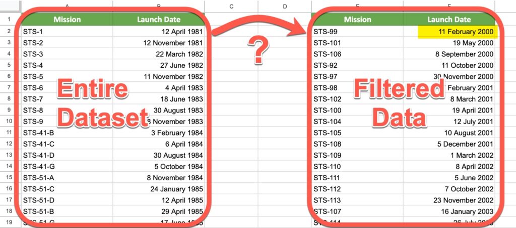
Suppose you have a dataset of Space Shuttle launches from the first launch in 1981 through to the final launch in 2011. You want to filter the data to look only at the subset from the year 2000 onwards.
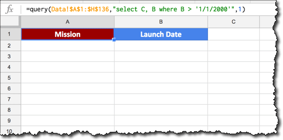
To begin, you might try the following syntax:
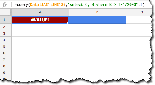
=QUERY(Data!$A$1:$H$136,"select C, B where B > '1/1/2000'",1)Unfortunately, the output of such a query is blank:
If instead we remove the single quotes from around the date and try again, we get a #VALUE! error because the Query formula can’t perform the comparison:
Alas, what are we to do!
Neither of these “standard” formats work, because the dates are not in the correct format for the Query function.
 💡 Learn more
Learn more about the QUERY Function in my comprehensive course: The QUERY Function in Google Sheets
Correct Syntax for Dates in the QUERY Function
Per the Query Language documentation, we need to include the date keyword and ensure that the date is in the format yyyy-mm-dd to use a date as a filter in the WHERE clause of our Query function.
Putting aside the Query function for a moment, let’s consider that "select..." string.
The new syntax we want will look like this:
date_column > date '2000-01-01'Our challenge is to create a text formula to create this syntax for us, inside our query function.
Dealing with the text function first, starting with our required date of 1/1/2000 and working outwards:
First, we convert it to a serial number format with the DATEVALUE() wrapper:
=DATEVALUE("1/1/2000")The output of this formula is a number:
36526Then the TEXT() function converts it to the required format for the Query formula by specifying a format of "yyyy-mm-dd":
=TEXT(DATEVALUE("1/1/2000"),"yyyy-mm-dd")The output of this formula is a date in the desired format:
2000-01-01Next we add single quotes around the new date format, with the "'" syntax. Finally, we insert the word date into the query string, to give:
="select C, B where B > date '"&TEXT(DATEVALUE("1/1/2000"),"yyyy-mm-dd")&"'"which gives or desired output:
select C, B where B > date '2000-01-01'That’s the syntax challenge done!
We can now plop that string into the middle argument of our Query function as per usual, and it’ll do the trick for us.
In this case, I was using a table of Space Shuttle mission data from Wikipedia, which contains a column of launch dates.
I used the IMPORTHTML() function to import that table into my Google Sheet, into a tab called Data in the range A1:H136. There’s a link to this dataset and worksheet at the end of the post.
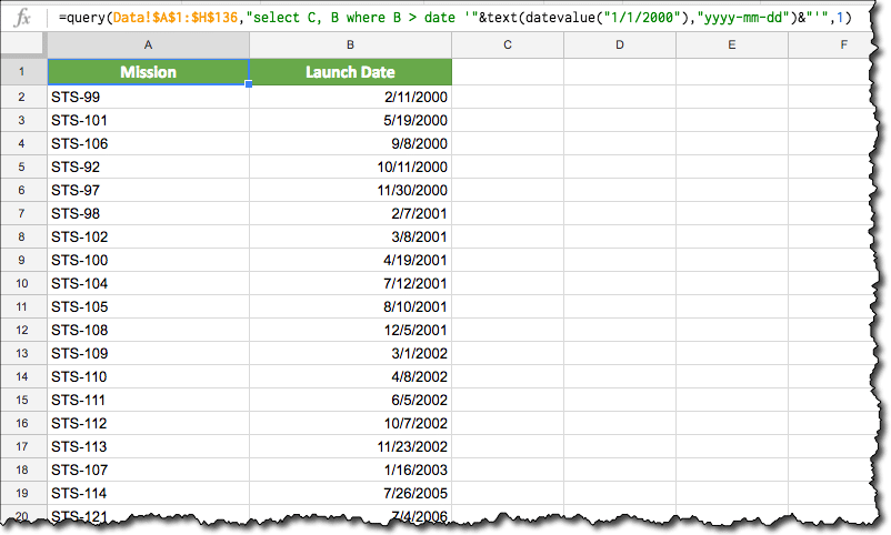
This Query formula returns all of the Space Shuttle missions after 1 January 2000:
=QUERY(Data!$A$1:$H$136,"select C, B where B > date '"&TEXT(DATEVALUE("1/1/2000"),"yyyy-mm-dd")&"'",1)The output of our formula is now returning the correct, filtered data:
Referencing a Date in a Cell
The formula is actually simpler in this case, as we don’t need the DATEVALUE function. Assuming we have a date in cell A1 that we want to use in our filter, then the formula becomes:
=QUERY(Data!$A$1:$H$136,"select C, B where B > date '"&TEXT(A1,"yyyy-mm-dd")&"'",1)Example Showing Filter Between Two Dates
Again, it’s relatively simple to extend our formula by adding a second date clause after the AND keyword:
=QUERY(Data!$A$1:$H$136,"select C, B where B >= date '"&TEXT(A1,"yyyy-mm-dd")&"' and B <= date '"&TEXT(B1,"yyyy-mm-dd")&"'",1)Today’s Date as a Filter
Substitute the TODAY() function into our formula:
=QUERY(Data!$A$1:$H$136,"select C, B where B > date '"&TEXT(TODAY(),"yyyy-mm-dd")&"'",1)Template
🔗 Click here to open a view-only copy >>
Feel free to make a copy: File > Make a copy…
If you can’t access the template, it might be because of your organization’s Google Workspace settings.
In this case, right-click the link to open it in an Incognito window to view it.