This article looks at how to add a total row to tables generated using the Query function in Google Sheets. It’s an interesting use case for array formulas, using the {...} notation, rather than the ArrayFormula notation.
So what the heck does this all mean?
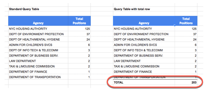
It means we’re going to see how to add a total row like this:
using an array formula of this form:
= { QUERY ; { "TOTAL" , SUM(range) } }
Now of course, at this stage you should be asking:
“But Ben, why not just write the word
TOTALunder the first column, and=SUM(range)in the second column and be done with it?”
Well, it’s a good question so let’s answer it!
The reason for using this method is because the total line is added dynamically, so it will be appended directly at the end of the table, and won’t break if the table expands or contracts, if more data is added.
It’ll always move up or down, so it sits there as the final row.
Simple example of how to add a total row
Before we get to the QUERY function example, let’s try a super simple one to understand the mechanics of the array formulas we’re going to be building.
Imagine I have this dataset:
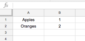
Like I said, keeping things simple.
Step 1: Combine tables using array
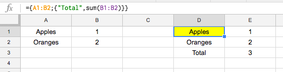
Let’s manually create a total row next to our original table, in cells D1 and E1, like so:
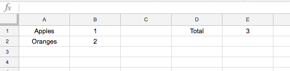
Then we can use this array literal formula, in cell G1, to combine these two tables into a single one:
={A1:B2;D1:E1}which, in our Google Sheet, looks like this:
The syntax is a pair of curly braces and a semi-colon to say the two tables should be combined vertically.
To that end, each table must have exactly the same number of columns.
Step 2: Create a total line using an array
Now, let’s use another array literal formula to generate that total line. Instead of typing “Total” into one cell, and a number into the adjacent cell, simply create the total line with a single formula:
={"TOTAL",3}The syntax is a pair of curly braces and a comma to say the two elements should be combined horizontally.
To that end, each original element must have exactly the same number of rows.
The array literal syntax is slightly different for European Sheets users. Check out this post: Explaining syntax differences in your formulas due to your Google Sheets location
Step 3: Use a SUM formula in total array table
Change the above formula to include a SUM function as follows:
={"TOTAL",sum(B1:B2)}Step 4: how to add a total row to the table with the array
Using the formula from Step 1, replace the second element in the array (the D1:E1) with the formula from Step 3, so your output formula is now:
={A1:B2;{"TOTAL",sum(B1:B2)}}This gives you your answer:
Step 5: Use indented notation in formula bar
This is purely a presentational step, to make the formula a little more readable inside of the formula bar. Simply add some line breaks (Ctrl + Enter) and indentations:
={

    A1:B2

  ;

    {

      "TOTAL",

      sum(B1:B2)

    }

  }
💡 Learn more
Learn more about the QUERY Function in my newest course: The QUERY Function in Google Sheets
Total row example with QUERY function
For this example we’ll use some New York City data, specifically data about how many open positions there are for different agencies within the city.
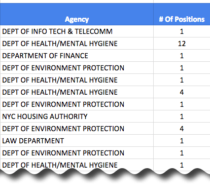
What we’d like to do is summarize the number of positions for each agency, i.e. combine all the agency lines into single lines with a total count for that agency.
We’re “grouping” our data into the categories listed in column A, and adding up all of the values in column B that fall into each group.
To achieve that, we use the QUERY function with a group by clause, to aggregate the number of positions data for each agency:
=QUERY($A$11:$B$61,"select A, sum(B) group by A order by sum(B) desc label sum(B) 'Total Positions'",1)which gives an output like this:
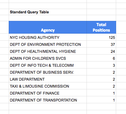
Ok, so far so good. Nothing new to see here.
(Learn about or refresh your memory on the QUERY function here.)
How do we go about adding that total row then?
How to add a total row:
Essentially what we’re doing is exactly the same as the simple example above, creating two separate tables (one is the summary table, like the one above, the other is the total row) and then we use an array formula to combine them into a single table.
Here’s a pseudo formula to illustrate what we’re doing:
= { QUERY ; TOTAL } <-- notice use of semi-colon ;
and then the Total is actually it’s own array formula as we saw:
{ "TOTAL" , SUM(range) } <-- notice use of comma ,
so that the final formula, a nested array formula, takes this form:
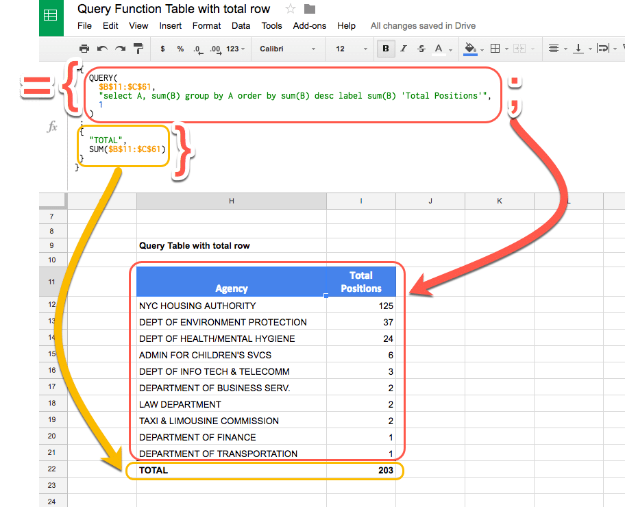
= { QUERY ; { "TOTAL" , SUM(range) } }So let’s go ahead and nest the QUERY function inside of the array formula, with an array SUM formula for the total:
={QUERY($A$11:$B$61,"select A, sum(B) group by A order by sum(B) desc label sum(B) 'Total Positions'",1);{"TOTAL",SUM($B$11:$B$61)}}(Optional) Let’s add some line breaks and indentations to make things a little clearer (you can do this in your formula bar too! Use Ctrl + Enter to insert new lines into your formulas and make them more readable):
={

  QUERY(

    $A$11:$B$61,

    "select A, sum(B) group by A order by sum(B) desc label sum(B) 'Total Positions'",

    1

  )

;

  {

    "TOTAL",

    SUM($B$11:$B$61)

  }

}
The following image shows how the different parts of the formula output data in the table, with the array syntax added in red:
Final step to make it dynamic
There’s one last tweak we need to make if we want it to be dynamic, so that the total row moves up or down as the table expands when we add or remove data, and exhibit behavior like this:
There are two things we need to do: 1) adjust the range to include whole of columns A & B, 2) adjust the QUERY function to remove the blank row that gets added after step 1).
Adjust the range by removing the $61 references so we include the whole of columns A and B. Then tweak the QUERY function by adding a WHERE clause to exclude all the blank rows from column A.
The final function is:
={

  QUERY(

    $A$11:$B,

    "select A, sum(B)  where A is not null group by A order by sum(B) desc label sum(B) 'Total Positions'",

    1

  )

;

  {

    "TOTAL",

    SUM($B$11:$B)

  }

}
What about if I have a WHERE filter clause?
Ah ha! Sneaky!
You need to add that same filter into the total calculation row, to ensure you’re only including the relevant values into your total.
Say for example, we wanted to only show rows beginning with DEPT then we’d use a LIKE filter in our WHERE clause, both the main one and the new one introduced in the total row:
={

  QUERY(

    $A$11:$B,

    "select A, sum(B)  where A is not null and A like 'DEPT%' group by A order by sum(B) desc label sum(B) 'Total Positions'",

    1

  )

;

  {

    "TOTAL",

    SUM(QUERY($A$11:$B,"select B where A like 'DEPT%'",1))

  }

}
Can I see an example worksheet?
Feel free to make your own copy.
Thank You! This is highly useful. Would one follow the same syntax if the query had two columns to sum? Would you be able to post an example of multiple columns to sum?
Yes, you can use the same syntax for more columns, you just need to be sure that the number of columns in your QUERY table matches the number of columns in your TOTAL row table.
Hi Ben,
Your site is incredibly helpful. Thankyou! I am struggling getting “Total” into my query below, what am I missing? I keep getting message ‘In ARRAY_LITERAL, an Array Literal was missing values for one or more rows.’ ???
={Query(‘2019’!$A2:$S, “Select H,I, sum (P) where I contains ‘”&$A$1&”‘ and A contains ‘”&$B$1&”‘ group by H,I order by sum (P) DESC limit 25 label sum (P) ‘Total Revenue'”,1) ; {“Total”, sum(Query(‘2019’!$A2:$S, “Select P where I contains ‘”&$A$1&”‘ and A contains ‘”&$B$1&”‘”,1))}}
Solved. Stacking Queries need to have same number of columns. If query returns no results you get the single column N/A message which is why I was receiving Array Literal error message. Solve by adding iferror( in front of query. Results if error set to bank columns equal to the number of columns:
={iferror(Query(‘Loan Timeline’!$A$3:$Q, “Select A,C,D,E where E > 14 order by D DESC”,1),{“”,””,””,””});
Hi Ben, sorry to write here because i couldn’t find the comment button :(.
what i want to ask about is can we combine query and running total?
for example i have beginning balances for each certain variables and then there are income and outcome amounts and i want to get running total as remain balance for each row in the query. And to the very end i want to add total as you introduced in this section.
hope you can understand my messy words, can’t wait to get this problem solved 🙂
Thanks
I am struggling with getting multiple columns to sum. This is what I currently have – no errors coming up, but no total row showing either: ={IFERROR(query(‘New Report Data Example’!$A$1:$V, “select B,A,G,N,O,P where B=’SampleA’ order by A asc”, 1),{“TOTAL”,SUM(query(‘New Report Data Example’!$A$1:$V, “select B,A,G,N,O,P where B=’SampleA'”,1))})}
If it matters, the only columns with numbers to sum are O and P (others are text or non-numbers).
Very useful…
Thank You for making my life easier
Fantastic post, thank you very match
Ben, many thanks for all those helpful tutorials!
One question, though…
Why don’t you put a “where A ” ” clause instead of the “limit” to not take the blank rows?
Wouldn’t that be better, allowing more ordering options in the results?
Good call Max D.!
Both solutions work, but I like using the WHERE clause because it’s less complex and relies on one less nested formula. Thanks. Have updated the article to reflect this.
I have more than just two rows and for some reason, it is saying:
1) That I have a circular dependency
2) Once I allow for one circular reference, it totals to 0
What’s your formula? Also, if you’re based in continental Europe, the “;” and “,” are the other way around…
={QUERY(Master,"Select B, sum(D), sum(E), sum(F), sum(G) Where A>= date '"&Text(B1,"yyyy-mm-dd")&"' AND A<= date '"&Text(D1,"yyyy-mm-dd")&"' AND("&Trim("upper(B) contains '"&Upper(JOIN("' OR upper(B) contains '",FILTER(G2:G,NOT(ISBLANK(G2:G)))))&"'")&") group by B label sum(D) 'Cost', Sum(E) 'Impr', sum(F) 'Inter.', sum(G) 'Conv.' " , 1); "Total",Sum(B3:B),Sum(C3:C),Sum(D3:D),Sum(E3:E)}Firduash – you need to add curly brackets {} around your total line, like this:
{"Total",Sum(B3:B),Sum(C3:C),Sum(D3:D),Sum(E3:E)}so your full formula becomes:
={QUERY(Master,"Select B, sum(D), sum(E), sum(F), sum(G) Where A>= date '"&Text(B1,"yyyy-mm-dd")&"' AND A<= date '"&Text(D1,"yyyy-mm-dd")&"' AND("&Trim("upper(B) contains '"&Upper(JOIN("' OR upper(B) contains '",FILTER(G2:G,NOT(ISBLANK(G2:G)))))&"'")&") group by B label sum(D) 'Cost', Sum(E) 'Impr', sum(F) 'Inter.', sum(G) 'Conv.' " , 1); {"Total",Sum(B3:B),Sum(C3:C),Sum(D3:D),Sum(E3:E)}}Hope that helps!
Ben
Hi Ben,
Unfortunately, it did not help. I still receive a circular dependency error. When I allow one iteration, it does not add, the totals row remains all zero. I tried adjusting the formatting of the raw data but that doesn’t make a difference. I used only two columns table to stay in line with your example but adding one column ends in a circular dependency or a 0 value.
Can you share your sheet? If I have time I’ll try to take a look. Cheers, Ben
Also, you need to sum the original data, not the data in the new query table, otherwise you’ll get circular dependency errors.
Hi Ben,
I had the same issue with circular dependency errors and found a hack.
={query(A:C,”Select A, Sum(B),Sum(C) where A is not null group by A order by sum(B) desc label sum(B) ‘Total Data1’, sum(C) ‘Total Data2′”);{“Total”, index(query(A:C,”select sum(B)”),2,1),index(query(A:C,”select sum(C)”),2,1)}}
I Basically query the Totals only and then wrap an INDEX around them.
Here is a link to the sample sheet https://goo.gl/rWK9NT
Hey Shane,
Thanks for sharing your solution, nice use of index 🙂
However, you shouldn’t get the circular errors if you’re summing the original data, with a straightforward sum formula.
Cheers,
Ben
Hi Ben,
Thanks for the positive feedback, and you right if you sum the original data you will not get a circular ref. The issue is sometimes your Query will have “filters” and summing the original data will not be accurate. Say you wanted to sum a range of data the contains the word “Dept” then your query will change and the therefore your totals will need to change too.
Great question!
Yes, absolutely. In this case you need to put a query filter inside of the SUM function in the total row as well. Taking your example of wanting to filter on the range containing DEPT, our formula for the total would look like this:
=SUM(QUERY($A$11:$B,"select B where A like 'DEPT%'",1))And the full QUERY with total row formula would look like this:
={QUERY($A$11:$B,"select A, sum(B) where A is not null and A like 'DEPT%' group by A order by sum(B) desc label sum(B) 'Total Positions'",1);
{"TOTAL",SUM(QUERY($A$11:$B,"select B where A like 'DEPT%'",1))}}
I’ve added this example to the article and template.
Cheers,
Ben
Hi Ben – I think your last example in the article may be missing a like statement in the first query function (the one that I’m replying to appear correct).
Cheers,
Stu
Good spot, Stu! I missed it in the main article. Updated now.
Cheers,
Ben
Hi Ben,
I’ve been trying to use this nice tip but for some reason it doesn’t work. I did change my spreadsheet settings “locale” from United States to Italy (for dates purposes, since I live in Italy) and doing so I did see my formulas change automatically their semicolons for commas. However, I tried your formula from this article to do vertical/horizontal arrays, and since I had “Formula parse error”, I tried the simple examples. I realized that ={“total”;3} works well as vertical array, but ={“total”,3} gives “Formula parse error”.
As a result, ={QUERY(‘Full database’!B1:BW;”select G,F,I,J where C contains ‘”&Corso&”‘ and D contains ‘Sí’ or D contains ‘sí’ order by F label I ‘Titolo'”;1), {“Total:”;COUNTIFS(‘Full database’!D3:D;”Sí”;’Full database’!C3:C;”Vesc 2017*”)}} gives me “Formula parse error” too…
So, if you would know anything, would be great!
Thank you,
Cédric
Hey Cédric,
You need to use a backslash instead of a comma in your array functions, so your formula would look like this:
={"total"\3}Cheers,
Ben
Thanks Ben. It worked great!
I had to add “”\””\ at the beginning of my array’s second parameter, since I have four columns in my query in my array’s first parameter. But anyways, I wouldn’t have figured out by myself the backslash \ trick.
Ben,
Thanks for all of the helpful examples. Unfortunately, I am not able to get this to work on my query which is below.
={QUERY({Donations!A:G; Payouts!A2:G}, “select Col1, sum(Col6) where Col1 != ” group by Col1 LABEL sum(Col6) ‘Balance'”); {“Total”, SUM($B$2:B)}}
I get a #REF! error for a circular dependency. Also when I tried SUM(Col6) I got a result, but the number was zero which is not correct. Any help you could provide would be greatly appreciated.
Best,
Kent
Hey Kent,
I think this may have something to do with the fact that your combining two data sources as your query table, but hard for me to tell without seeing the data.
The way I always figure these out is to just set aside the query function and figure out the plain SUM function in a separate cell. Once you have that working you should be able to plug it into your {} formula.
Cheers,
Ben
Have you found a way to do the total with a pivoted set of values, say 9 different queries for a sales activity by day of the month (they have to be separate queries to plug in a fix set of sales stages so blank/zero returned values are also shown). Is there is no alternative to totaling queried values across multiple queries?
Scratch that question, regular totals are working for me on multiple queried values. Great, informative post!
Great you got it sorted!
I’m doing something similar. I am returning a dynamic set of data, pivoted by date column to include a variable number of columns equaling the number of dates between the user selected date range. So the number of rows AND columns will be variable. I would like to have a total column at the far right for each row, AS WELL AS a total row totaling each column. Can this all be done all together for a nice compact data view? Thanks!
How can I do a vlookup from a query? Say, I query a range and base individually lookup a value from another database. Is there anything like inner join in VBA world?
There’s no JOIN functionality in the Query function, but there are some workarounds out there: https://stackoverflow.com/questions/48166016/how-to-join-tables-using-query-or-vlookup
Hello!
Trying to get this to work for my amateur attempt at a sheet.
Can someone take a look at this file and reccomend how to get the query and the dynamic total line to work? I essential want to query portions of the tab named “Markup”, I’ve applied a name to that range to make it easier to reference.
The query is on tab “Summery Tab” and is in cell A3. It functions currently as a straight query, but I can’t seem to integrate the above method of applying a dynamic total line.
Thanks!
Here’s the link to the doc…
https://docs.google.com/spreadsheets/d/1S-8PcH18yuu-QfaprxWM9kKhhhRc3Bd-QVda4TMfWs4/edit?usp=sharing
Edit permission is on, but please leave me comments/notes on how it was fixed.
Error
In ARRAY_LITERAL, an Array Literal was missing values for one or more rows.
={query(projects, "select Q,R,S,T,U,V,W,X,Y where Q="&B1&"");{"TOTAL",SUM(I24:I)}}Same here:
={QUERY(
projects,
"select Q,R,S,T,U,V,W,X,Y where Q="&B1&"",
1
)
;
{
"TOTAL",
SUM($I$24:$I)
}
}
Hi Ben!
I have a data validation cell (Sheet1 B1) that I reference, and a named range (Sheet2 ‘projects’). Could you explain why this formula is returning an error and how I can fix it? Column Q is the product ID, and column Y is the cost. I’m trying to replicate a pivot table that I can filter via the data validation cell.
={query(projects, "select Q,R,S,T,U,V,W,X,Y where Q="&B1&"");{"TOTAL",SUM(QUERY(projects,"select Y where Q="&B1&""))}}This forumla returns #VALUE ‘Error
In ARRAY_LITERAL, an Array Literal was missing values for one or more rows.’.
Thanks in advance!
Hi Micah
It gives the error cause your arrays dont match. You need to add a few cells to match them.
Ex.
={query(projects, “select Q,R,S,T,U,V,W,X,Y where Q=”&B1&””);{“”,””,””,””,””,””,””,””.”TOTAL”,SUM(QUERY(projects,”select Y where Q=”&B1&””))}}
Hope this helps
Thanks, i’ll write in a fee minutes, I really apreciate this page!
:):)
Nancy
Hey Buddy,
thanks for this, it’s very clever & useful.
what if you have a query that uses import range? is there a way around that?
Ben, Love the blog and am working my way through your paid for courses. Excellent value.
I’m trying to format a total:
={query(AllTransactions, “select O, sum(D)*-1 WHERE C='”&B1&”‘ group by O LABEL O ‘Project Name’, sum(D)*-1 ‘Balance’ FORMAT sum(D)*-1 ‘£#,##0.00′”,);
{
“TOTAL”,
SUM(QUERY(AllTransactions,”select D*-1 where C like ‘”&B1&”‘ FORMAT D*-1 ‘£#,##0.00′”,1))
}
}
is there something obvious I am doing wrong? Thanks
Hi Ben, thanks for this awesome article! When I add line breaks as you describe in your article for readability, it works great. However, when I try to add indentations by hitting the space bar a few times, the indentations do not save (the content all goes back to be left justified with no indentation). How do you add the indentations?
Thanks,
Adam
this no work ?? = {
QUERY
(
OPERACIONES;
“Select B,E,F,G,H
where F ='”&D3&”‘
and D = ‘Ingreso’
and C >= ‘”&E1&”‘
and C <= '"&E2&"'";
-1);
{"example","example","example","example","example"
}
}
OPERACIONES; —>OPERACIONES,
Hi Ben,
Thanks so much for this! It’s amazing and works like a charm. I found your advice to build the formulas separately and then combine them to be particularly helpful.
I have this up and running and it’s working great. I’m now trying to refer to cells in my ‘Total’ line in order to make calculations, with the Total often being an absolute reference in my formulas (i.e. % of Total). Do you know if there’s a way to make that absolute reference dynamic so that it will change if the total line changes positions due to changes or additions in the data? I realize this may not be possible, but thought I’d ask… Appreciate any advice you have.
Dunno if you’re still wrestling with this, but here’s a suggestion:
use
MATCH(“Total”,Sheet!:,0)
to find what row the Total label is in, then
INDEX(Sheet!:,,1)to get the value from the column with the total amount, for example:
=INDEX(Data!H4:H,MATCH(“Total”,Data!A4:A,0),1)
which assumes the label “Total” is in Data! Column A and the actual total amount in Data! Column H.
Fantastic tutorial! It worked like a charm!
Just one question, though: if you make the total row dynamic, how do you give the total row special formatting to distinguish it from the other rows?
Hey Nate, did you figure this one out?
Hey Nate and Raj,
I figured it out. Basically highlight the whole potential range, add a custom format (via right click or menu), make the format rules use a custom formula and put this in it. Note the 1 is misleading, it just means the row being evaluated (it should be the same row your custom format row starts on). Then you can bold, color it etc.
=$A1=”TOTALS”
I have some comments which are static in corresponding rows . When data is added the rows get added but comments remain same .
Is there any way to use the sum of the output column as a label for that column?
For example, instead of stating
“label sum(B) ‘Total Positions”, I want to state
“label sum(B) ‘sum(Col3)’.
I’ve messed around with this concept but it doesn’t seem to produce the result I want. Is this possible?
Hi Ben
I have a sheet with raw data which is populated by a form with oldest date at the top
I then use the query function to select data and out put it to tabs
In one tab I add a calculation to each row of cells in a column at the side of each row. The function sits in each cell at the end of the row and is not part of the query
Example: The tab data relates to reported faults. I use the data validation function to allow the user to indicate whether the fault is “sorted” or “open” which could be at some future date
As people access the information on cellphones it would be preferable to have the data in “newest” date first which I can order through the query
However as the query is a dynamic function it would break the sequence by inserting a new row without the additional function in the cell at the end of the row
Question. Is there a way of achieving this or do I accept the date order is oldest first?
Thank you very much
Hi Ben
Further to my original question, I have done some experimenting and found that by importing the original raw information into a tab using the query function AND THEN importing it into a second tab using a suitable query function to get the right data I can set the ORDER to be “newest” first and the additional data validation function is not broken.
This does mean that data cannot be erased or the data will become out of sync
So please may I modify my question and say is there a more efficient way of doing this
Hello Ben,
Just a tricky question. My total row is adding up spendings, that is, it is should be, if possible, formatted as currency number.
How can I achieve this? Any idea? Thanks.
Cedric
Hi,
currently my formula wont work if my select column are to many,
if i remove SUM(I) on my formula it works.
={QUERY(‘JOIN-SALES-DB’!A1:N,”SELECT B,C,D,E,G, SUM(H),SUM(I) WHERE F = ‘”& B5 &”‘ GROUP BY B,C,D,E,G”,1);
{“”,””,””,””,”TOTAL”,SUM(QUERY(‘JOIN-SALES-DB’!A1:N,”SELECT SUM(H),SUM(I) WHERE F = ‘”& B5 &”‘”,0))}}
Hi Ben,
You are a life saver and I love the blog and your courses! What I’m having issues with is the following:
I have a table which gets bigger every week. I want to use an ArrayForumla to sum the items in each column that have the same heading.
A B C D E F G …… NW NX
Week 24-10 Week 17-10 Week 10-10 Week 3-1
Name Hours FTAR# Hours FTAR# Hours FTAR# Hours FTAR#
Mr. X 23 7 36 4 38 5 37 9
Mr. Y 36 6 23 6 39 6 41 8
Mr. Z 35 5 35 5 36 5 39 6
This is easy with SUMIF i.e. SUMIF(A2:NX2,”Hours”,A3:NX3) but this table has a LOT of rows and hence each Total column has a corresponding SUMIF formula. Surely there’s an easier way with =ArrayFormula{SUMIF(??????????????????????????)} or ArrayFormula{(DSUM(????????????????)}.
This ‘should’ be trivial but for me, it’s proving anything but.
With this code it is possible to edit a cell in the original database or it is only for consultation?.
Hi,
How do you insert a blank row befor TOTAL in your example?
Ben, you seem pretty savvy with query so I wanted to see if you could answer the following: I want to know the difference from previous date in a query pivot row. Example is: count the number of days between operator errors. I can almost get there in excel with calculated fields using difference from previous but I’d prefer this in a gsheet and difference from previous is not an option in gsheets yet. Any chance this can be done in a query?
Hi Ben.
I appreciate your contribution to Google sheets. I am facing a peculiar problem while using ORDER BY clause in QUERY. The numbers are showing as 1.1, 1.2, 10.1, 11.1 and then 2.1.2.2 so on.
How to ensure that the sort order is maintained.
Hi, thanks a lot for this post. Was very helpful.
Quick question: is it possible to add, i.e.: skip – one row before the total?
Thanks
Hi, leaving a reply for everyone from countries that use commas as separators, this is how you add a total row:
={
QUERY(A10:D26; “SELECT C, SUM(D) WHERE D 0 GROUP BY C)
;
{
“Total”\
SUM(D10:D26)
}
}
The ; will add rows (vertically adjoin the arrays) and the \ will add columns (horizontally adjoin the array values).
@Esteban Martinez
Sure, taking my previous example, simply add empty values. You can either add a new empty subarray or just add the values in the same array. Subarray with 1 row with empty values: Hi, leaving a reply for everyone from countries that use commas as separators, this is how you add a total row:
={
QUERY(A10:D26; “SELECT C, SUM(D) WHERE D 0 GROUP BY C)
;
{
“Total”\
SUM(D10:D26)
}
}
={
QUERY(A10:D26; “SELECT C, SUM(D) WHERE D 0 GROUP BY C LABEL C ‘Budget’, SUM(D) ‘Points'”)
;{“”\””};
{
“Total”\
SUM(D10:D26)
}
}
And the same example, but with the values added into the Total array: ={
QUERY(A10:D26; “SELECT C, SUM(D) WHERE D 0 GROUP BY C LABEL C ‘Budget’, SUM(D) ‘Points'”)
;
{“”\””;
“Total”\
SUM(D10:D26)
}
}
So in short, all you need to do is add one or as many rows with as many empty values as there are columns.
Great post. I there a way to make the query subtotal so that different groups have a total row beneath them?
I can’t seem to figure out what I’m doing wrong here:
={
query(
‘Fall 2020 All Enrollment Records’!A2:N,
“Select I,E,D,F,G,H,N where E is not null and C contains ‘”&B2&”‘ order by I,F”)
;
{
“Total”,
SUM(QUERY(‘Fall 2020 All Enrollment Records’!A2:N,”Select N where C contains ‘”&B2&”‘”))
}
}
Oops, never mind. I realized now that “Total” counts as 1 column and the Sum counts as another. So if I have 7 columns in the first query then I need to add 5 blank columns prior:
{“”,””,””,””,””,”Total”,SUM(stuff)}}
Thank you Ben and Nick and others, this is very helpful.
Brilliant, thank you very much for giving such a detailed explanation. This post is somehow old but it keeps on being userful.
Thanks
It was a nice representation of Google Script Query. Got a lot of new info. Thanks Ben.
I wanted to generate a query table and a item total below the query table. As you had mentioned I could have separately generated the total table but it creates problem when new lines are added in the source.
My original table have headers Date, Item, Credit and Debit. I select a few records from the original table through query. That works fine. I wanted to add item-wise total at the end of the table. I am facing the following problems:
1. Date column should be left blank in the total query table.
2. I want to supress the header for total columns.
3. At the end of the item total table, I wanted to add a grand total line also where Date column should be left blank and “Total” should be added to “Item” column.
Can you suggest some solution or provide links from where I could get it?
Regards,
Pravin Kumar.
can this be done using a Importrange inside of query?
Hi Ben,
I need some help regarding query function in google sheets.
I have data set with different items and quantity of each items.
All items will have sub item color and quantity as well.
Now i want to use the query function which gives me output greater to smaller of total of each item.
Data set
Item name | Color | Qty
Apple | Red | 2
Apple | Green | 2
Apple | Red | 5
Mango | Yellow | 3
Mango | Green | 5
Desired output
Apple | Red | 7
Apple | Green | 2
Apple Total | 9
Mango | Yellow |3
Mango | Green | 5
Mango Total | 8
Now, in above output total of apple is 9 so it will come first and then mango.
I love this solution but am struggling to apply it. Everything is working except I can’t get this Total row to appear. I need the option where there is a WHERE condition. To get the table to appear correctly this is the query I have used:
={
QUERY(MergedData,
“select M,J,avg(V),sum(T),avg(W) where J is not null AND G=’GfK’ AND Q=’1′ AND E=”&X2&” group by J,M order by M,J”,
1
)
}
I need to see sum totals for 3 columns: V, T and W.
Can you please help with the portion of the query string that would add the total row in for these (it needs to be able to expand/contract as the number of rows in the source data will change)?
Thanks
Kevin
={
QUERY(QUERY(A22:Q, “SELECT A, COUNT(A) WHERE A IS NOT NULL GROUP BY A PIVOT C”, 0), “SELECT * WHERE Col1 IS NOT NULL”, 0),
QUERY(QUERY(A22:Q, “SELECT COUNT(A) WHERE A IS NOT NULL GROUP BY A PIVOT D”, 0), “SELECT * WHERE Col1 IS NOT NULL”, 0),
QUERY(QUERY(A22:Q, “SELECT COUNT(A) WHERE A IS NOT NULL GROUP BY A PIVOT E”, 0), “SELECT * WHERE Col1 IS NOT NULL”, 0)
};
{“TOTAL”, SUM($B$2:$B), SUM($C$2:$C), SUM($D$2:$D), SUM($E$2:$E), SUM($F$2:$F), SUM($G$2:$G)}
}