How To Create Arrays In Google Sheets (a.k.a. Array Literals)

Arrays in Google Sheets are collections of data, consisting of rows and columns. You can use arrays in formulas in the same way that you use regular A1-type ranges.

You construct arrays in Google Sheets with curly brackets: { }

They’re also known as ARRAY LITERALS.

How To Create Arrays In Google Sheets

Row Array

Let’s start with a very simple row array example:

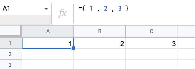
The formula to create this array, in A1, is:

The opening and closing curly brackets denote the array.

Commas separate the data into columns.

(Note, if you’re a European user, you use a backslash as the column separator. Read more about syntax differences in your formulas due to your Google Sheets location.)

Column Array

Now consider this column array:

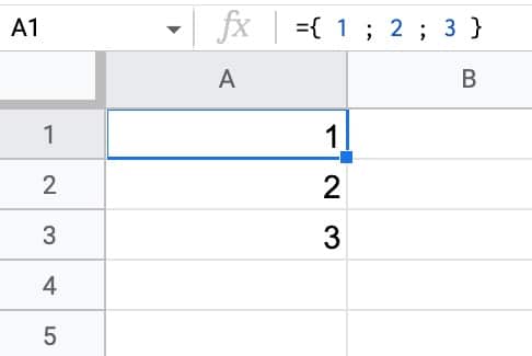
where the formula is:

Here, semi-colons create new rows in the array.

Two Dimensional Array

Next, consider this example:

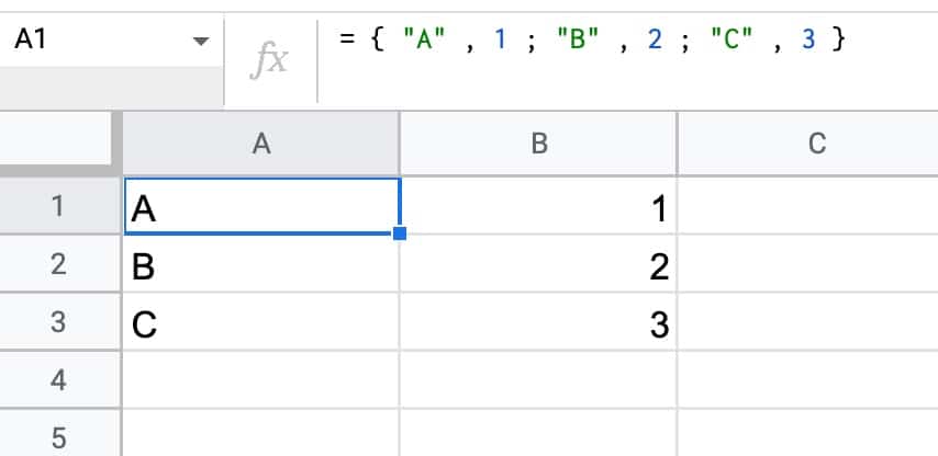
This formula, entered into cell A1, creates a 3 by 2 array that puts data in the range A1:B3:

You can see the combination of curly brackets to create the array, commas to create columns, and semi-colons to create new rows.

Array Literal Notes

You’re not limited to numbers or strings inside the array literals. You can also nest formulas inside the curly brackets, even array formulas. And when you combine formulas inside array literals, you unleash their full power.

Moreover, you can use the outputs of arrays as inputs to other formulas. See below for examples.

Read about arrays in the Google documentation.

Note, there are also other ways to create array outputs, for example, the SEQUENCE function can generate row, column, or 2-d ranges of data.

Examples Of Arrays In Google Sheets

Now that you’ve seen how to create arrays, let’s look at how to use them for practical applications in formulas.

Return Multiple VLOOKUP Columns

With a regular VLOOKUP formula, you’re restricted to returning a single column.

However, if you nest an array literal as the column index, you can return multiple columns at once.

Have a look at this example:

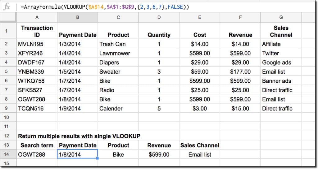
Notice the array literal nested inside the VLOOKUP, shown in red:

This VLOOKUP will return results from columns 2, 3, 6, and 7 simultaneously.

Read more about using Vlookup To Return Multiple Columns In Google Sheets.

Combining Formulas in Arrays in Google Sheets

One of the differences between the powerful QUERY function and a Pivot Table, is that the QUERY function doesn’t add a total row by default.

But you can use these arrays in Google Sheets to easily add a dynamic total row.

Essentially, you combine the results of the QUERY function with a SUM function:

which looks like this in your Google Sheet:

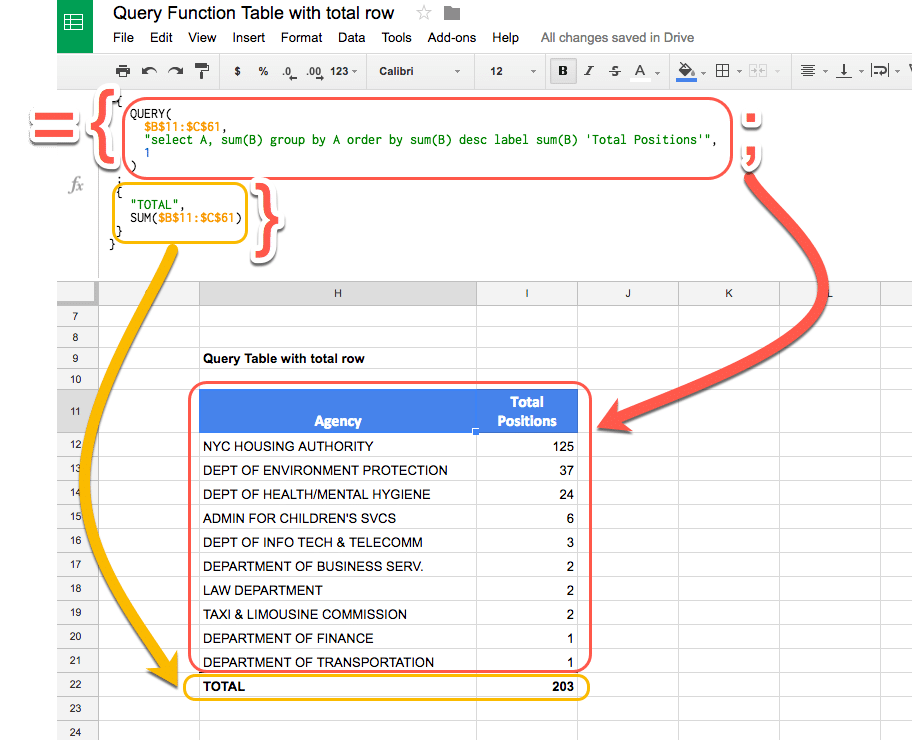
Read more on how to add a total row to a Query Function table in Google Sheets.

Default values for cells in your Google Sheets

You can also use arrays in Google Sheets to create default values for cells in Google Sheets.

The array literals create a formula that spills into the adjacent cell. This property is used to create a default value.

Let’s see an example.

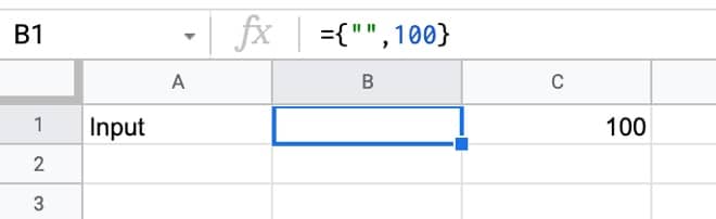
In a blank Sheet, write the value “Input” in cell A1. In cell B1, type this formula:

Your Sheet will look like this:

Try typing 200 in cell C1, over the top of the 100.

Cell C1 will show the 200, but cell B1 now displays a #REF! error.

Now, delete the value you just typed in cell C1. The error message disappears and the default value of 100 is displayed again.

Finally, hide column B so that the #REF! error is never seen, and you have a default value of 100 set for cell C1.

Read more about default values in Google Sheets, including a more advanced method to create default values without requiring a hidden column.