In this post, you’ll learn how to set default values for cells in Google Sheets, without using Google Apps Script code.
In the Sheet below, the cells in column B have default values of 100, 25, and 10 respectively. If a user types in a value (e.g. 200) it overwrites the default value. If a user deletes whatever value is in the cell already, then the default value of 100 is displayed again.
Setting Default Values For Cells In Google Sheets
The key to make this technique work is to use Array Literals to create a formula which spills into the adjacent cell. This is a rather abstract concept, so let’s run through an example.
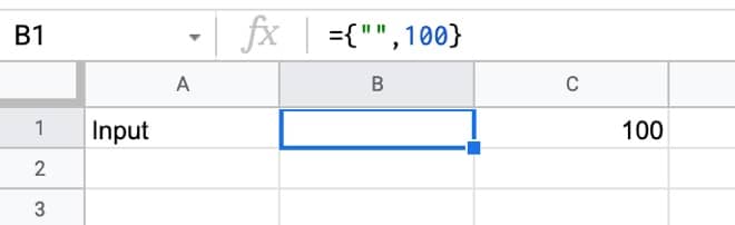
In a blank Sheet, write the value “Input” in cell A1. In cell B1, type this formula:
={"",100}Your Sheet will look like this:
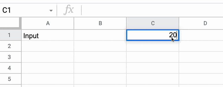
Try typing 200 in cell C1, over the top of the 100.
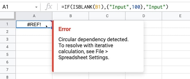
Cell C1 will show the 200, but cell B1 now displays a #REF! error.
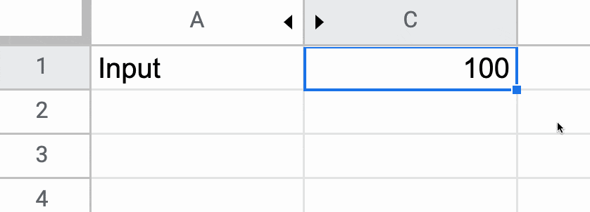
Now, delete the value you just typed in cell C1. The error message disappears and the default value of 100 is displayed again.
Finally, hide column B so that the #REF! error is never seen, and you have a default value of 100 set for cell C1.
🎩 Hat tip to my friend Scott Ribble for showing me this ingenious solution.
Advanced Default Values Without Hidden Column
The method above suffers from one drawback though: it necessitates a hidden column.
However, we can use a clever circular formula to address this.
In a new blank Sheet, add this formula in cell A1:
=IF(ISBLANK(B1),{"Input",100},"Input")Initially, you may see this error message about a circular error (i.e. a formula that references itself):
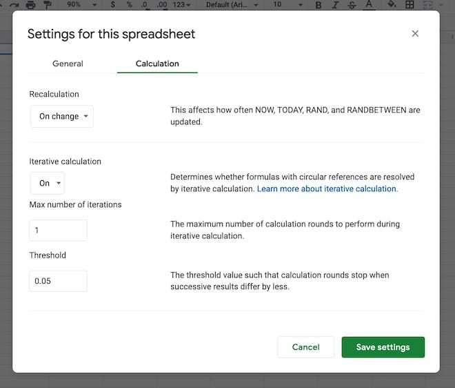
That is a problem, but we fix it by switching on iterative calculations and restricting them to a single iteration from the menu:
File > Settings
Go to “Calculation”.
Set “Iterative calculation” to “On” and the “Max number of iterations” to 1.
(The threshold can be left at 0.05 because it doesn’t apply in this case.)
Now, you can enter any value you want in cell B1 and if you delete it, the default value of 100 will be shown.
How Does This Work?
The IF function checks whether cell B1 is blank.
If it is blank, then it outputs the array literal:
{"Input",100}which displays “Input” in cell A1 and the value 100 in cell B1.
However, if cell B1 already has a value then the IF function output is just the string “Input” in cell A1.
Note: default values are not limited to numbers. It could be text, an image, or even another formula.
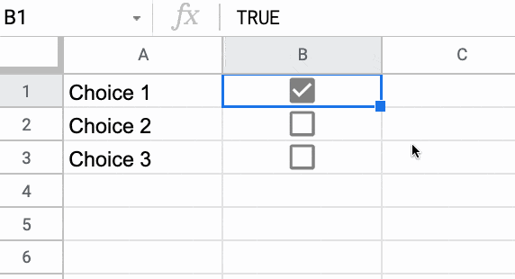
Default Values Checkbox Example
You can use default values to check or uncheck checkboxes. Here’s a cool illustration of how to create a select all checkbox in Google Sheets, using deafult values.
Thanks to one of the readers in the comments below for sharing this solution.
Default Values Formulas To Mimic Radio Buttons
Another interesting use case for these default values is to mimic radio buttons with formulas and checkboxes.
Column A contains array literal formulas that ensure a user can only select a single checkbox at a time.
Does the formula,
={"",100}, always refer to the cell directly to the RIGHT of it?Hi Cathy,
Yes, it does. You can specify the cell below by using a semi-colon instead of the comma, e.g.
={"";100}(Note, the syntax for the array literals is different if you’re based in Europe because of the Sheets location.)
You could also skip columns by setting the formula to be e.g.
={"","",100}But then you have two blank/error columns to watch out for.
Cheers,
Ben
Thank you so much Ben..
Thanks for the “hat tip” Ben!
I agree that hiding columns can be a drawback. I do think there are cases where they can also be very effective though, like when building tools for non-spreadsheet savvy people. When building sheets for others, I can think of at least 3 other benefits from using array literals and hidden helper columns.
1. I can protect labels and formulas from being overwritten accidentally.
2. I can hide alarming error messages and supply users with helpful instructions instead.
3. I can add notes to myself within the formula.
Here’s an example to illustrate with a blank sheet:
IN A1 ENTER:
={"Hidden Formula Column with formula notes","Label","Hidden Formula Column with formula notes","Value","Hidden Formula Column with formula notes","Helpful Instruction Message"}IN A2 ENTER:
={"Label","Input"}IN C2 ENTER:
=iferror({"Default Value",100},"default value overwritten")IN E2 ENTER:
={"Check if A2 or C2 is an error and tell the user what to do to fix it.",iferror(ifs(
iserror(A2),"Label was overwritten. Select cell B2 and press DELETE to refresh",
iserror(C2),"Value overwritten. Select cell D2 and press DELETE to refresh"))}
Set conditional formatting for B2 as
=iserror(A2)Set conditional formatting for D2 as
=iserror(C2)Then hide columns A, C, and E.
The result will be a visible table where any bad data can simply be deleted to restore default functionality and formulas with notes are a little more safely concealed.
Thanks for sharing, Scott! These are some great ideas.
Hi Ben (et al),
I find it works a little better with a SPLIT() like this:
=IF(LEN(B1),”Input (manual)”,SPLIT(“Input|100″,”|”))
Nice idea, Matt! Thanks for sharing.
I was wrestling with how to set the value of a cell once, based on an initial condition, and then have the value persist when that condition failed. I did not think it was possible to have a cell refer to itself, so I did not try it until I came across this thread.
Although I did not use the method shown, with an array, it pointed the way to success.
The following is the contents of L16. E20 and P20 are both initially 13. When both of the IFs fail, the false result is set to itself.
=IF(AND(E20=12, P20=13), B1, IF(AND(P20=12, E20=13), M1, L16))
Thanks for your site.
Great stuff, Len! Thanks for sharing your findings.
As an addendum to what’s described in the article, it’s possible to use the same idea (which I guess could generically be described as controlling the length of a dynamic array based on a conditional) to control tickboxes in a way which mimics the sort of thing which has traditionally required Apps Script. The key to doing this is to use the ‘use custom cell values’ option for tickboxes in the ‘Data validation’ menu to set unticked boxes to a blank value rather than ‘FALSE’ which has to be done in the slightly hacky way I’ve described below. Strategically placed IFs can then be used to control the tick boxes in various ways; a basic example is to create a ‘master tickbox’ which sets a range of other tickboxes all to true at the same time. For example:
1. Select cells A1, A3 & A4 and insert tickboxes via Insert/Tick box
2. Select A1 then go to Data/Data validation, tick ‘Use custom cell values’ and set ‘Ticked’ to TRUE and ‘Unticked’ to a single quote (‘). Repeat the process for the A3:A4 range.
3. If you highlight a unticked tickbox cell without ticking the box, you should be able to see that the formula bar contains a single quote character for the unticked boxes.
4. Select cells A1, A3 & A4 once again, and tick and untick them all using Space. You should now see that the formula bar is blank for the unticked boxes.
5. Enter the following formula in A2:
=if(A1,{"";TRUE;TRUE},"")(N.B. you may need to change the array literals depending on your locale)The tickbox in A1 now ‘controls’ the tickboxes in A3 & A4 by placing TRUEs in them every time you tick A1, and removing them every time you untick A1. Proviso: if A3 & A4 are set by ticking A1 they can’t directly be unticked (as they are now being set by the result of a formula), they must be unticked through A1 (so it’s not quite as good as an Apps Script based solution). More complex controls are possible with more IFs running in the column to the left of the tick boxes (as dynamic arrays spill rightwards and downwards); I’ve managed to enforce a maximum of two ticks in a range for instance, and I’m sure other significantly more complex controls might be achievable too.
Wow, this is cool. Thanks for sharing. I’ve played around and got a version working.
If you extend your formula, you can theoretically check as many boxes as you wish, e.g.
=if(A1,{"";TRUE;TRUE;TRUE;TRUE;TRUE;TRUE;TRUE;TRUE;TRUE;TRUE},"")checks/unchecks ten boxes in range A3:A12.
Great work!!
To follow up…
I wrote this method up in post: https://www.benlcollins.com/spreadsheets/google-sheets-select-all-checkbox/
Cheers!
I’m having a lot of trouble getting this to work stably. First case: using the formula on one line. It mostly works, but some actions, like copy-pasting into nearby cells (even in columns to the left!) will cause the state to suddenly switch.
Second case: formula on multiples lines. Now nothing works. Changing the value in one cell makes the state flip in all the subsequent rows, even though the formula never refers to any other cell.
Here’s a sample spreadsheet where I’ve set up examples: https://docs.google.com/spreadsheets/d/1yqrmafywyJpaGVUwKXGNetTbr1RveuT00GtJSOwY5ts/edit?usp=sharing
In the ‘single row’ sheet, try copying cell A2, for example, and pasting it into A4. B2 will briefly flip from “not selected” to “selected”.
Then look at the ‘multiple rows’ sheet. It’s just baffling.
Thanks for your help!
Hi ben, thanks for your great work!
Would this work with an array?
Let’s say I’d like an entire column to be editable and also have a default value (based on a set of ifs) if no custom value was entered.
But the arrayformula would then return a REF error because it can’t overwrite the custom value.
So overwriting the default value would not only effect that cell, it would effect the entire array. Not good.
Any other solution?
Great trick. I’ve used it many times.
I was wondering: is there anyway to use the first method with an array formula so that I don’t have to drag formula you have in colB down and colC defaults each row to whatever the arrayformula would output?
This is a nice solution, but I wish it would continue to work when you add new rows :(.
Hi Ben
Thanks for the thread!
I am looking for whatever data we typing in C1 will be overwrite by this default value, please help me on this function, Thanks Ben!
Hi,
When i writing with the comma, it comes with an error, but i works with simicolon, can anyone help with this
Best regards and thanks
Philip
Hi Philip,
Sounds like it might be a syntax location error. Have a read of this post: https://www.benlcollins.com/spreadsheets/sheets-location/
Cheers,
Ben