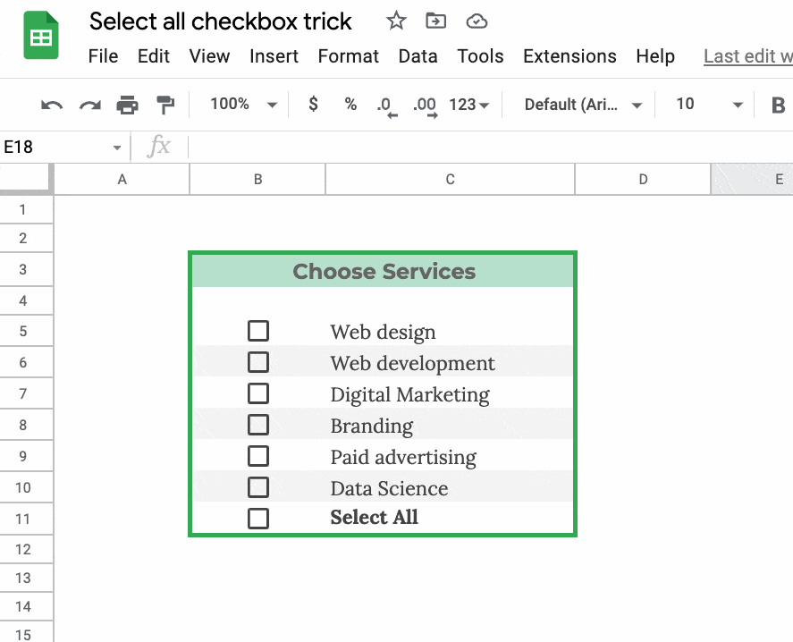
In this post, you’ll learn how to create a Select All checkbox in Google Sheets, as shown in this image:
But before we look at that, did you know there’s already a quick way of selecting all checkboxes manually?
Select All Checkboxes With Spacebar
Highlight a range of checkboxes.
Press the spacebar to toggle them checked or unchecked.
How To Create A Select All Checkbox in Google Sheets
Ok, onto the good stuff then 😉
And firstly, I want to tip my hat to one of my readers for sharing this technique with me. Thank you, God of Biscuits, whoever you may be!
Alrighty then! Let’s see how to create that select all checkbox in Google Sheets.
This technique combines checkboxes, setting default values with array literals, and conditional formatting across one row.
Let’s set it up in column A, without all the bells and whistles, so that you can see how it works.
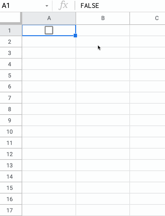
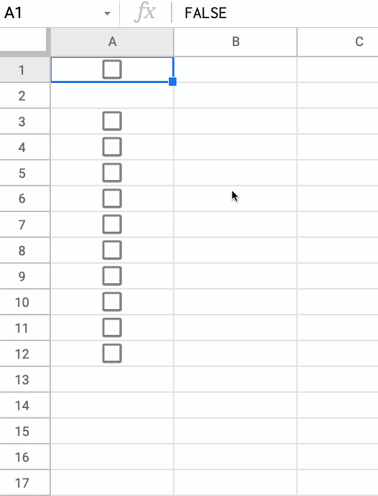
Step 1: Add the main checkbox
Insert a regular checkbox into cell A1, from the menu: Insert > Checkbox
Step 2: Add the secret formula
Copy this formula into cell A2:
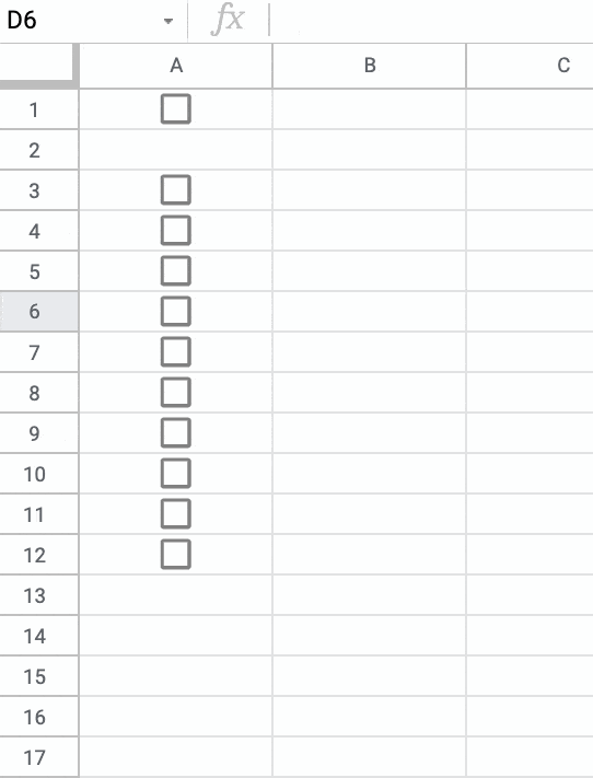
=IF(A1,{ "" ; TRUE ; TRUE ; TRUE ; TRUE ; TRUE ; TRUE ; TRUE ; TRUE ; TRUE ; TRUE },"")Toggle the checkbox and you’ll see the formula outputs 10 true values in the range A3:A12, like this:
The formula uses an IF function to check whether the checkbox in cell A1 is checked (TRUE) or unchecked (FALSE).
If it’s checked, then it outputs an array literal of 10 true values.
If it’s false, i.e. unchecked, then the formula simply gives a blank output.
You can probably see how it fits together now. We need to add some checkboxes to those cells A3:A12.
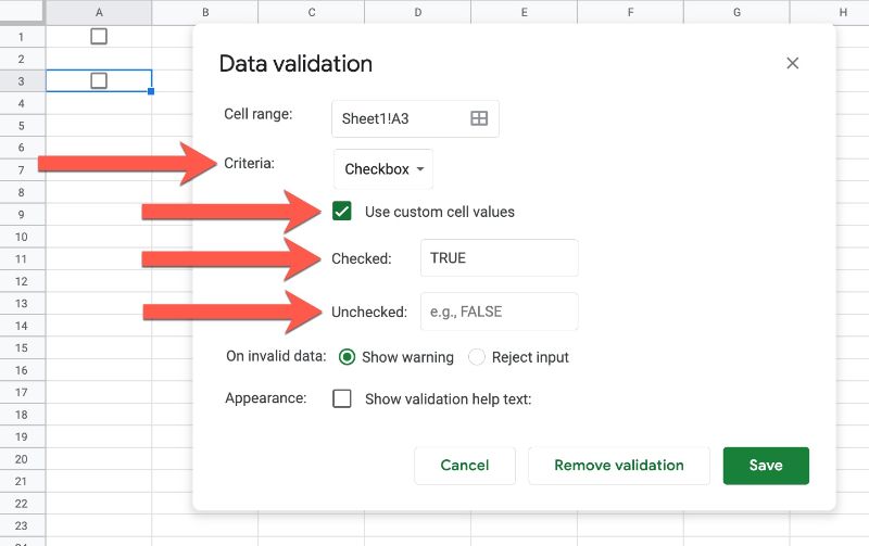
Step 3: Add the first special checkbox
Go to cell A3 and add another checkbox through the Data menu: Data > Data validation
Under Criteria, select the checkbox.
Then select “Use custom cell values”
Set the TRUE value to be TRUE.
Set the FALSE value to be a blank cell (ignore the e.g. FALSE suggestion in the box already).
Step 4: Add remaining checkboxes
Copy and paste this new checkbox from cell A3 to the range A4:A12.
Now, when you check or uncheck A1, all the checkboxes in A3:A12 will automatically be checked or unchecked.
Step 5: Formatting
To make the example at the top of the page, have a look at these two articles for instructions:
- How To Apply Conditional Formatting Across An Entire Row In Google Sheets
- Checklist Template In Google Sheets
Notes On The Select All Checkbox in Google Sheets
This method suffers one major drawback.
The select all checkbox only works when the checkboxes are unselected. In other words, once a user selects one or more of the checkboxes then the main select all checkbox won’t work.
You get a #REF! error if you try to use the select all when you already have some checkboxes selected.
Select All Checkbox in Google Sheets Template
Click here to open a view-only copy >>
Feel free to make a copy: File > Make a copy
If you can’t access the template, it might be because of your organization’s Google Workspace settings. If you right-click the link and open it in an Incognito window you’ll be able to see it.
See Also: How To Mimic Radio Buttons With Formulas And Checkboxes
Another interesting checkbox technique is to mimic radio buttons with formulas and checkboxes.
You use array literal formulas to ensure a user can only select a single checkbox at a time.
Wow, that was quick! Explained much better than me as well… I’m surprised that the hacky single quote in the FALSE field isn’t required; I could swear it was needed when I first tried this as the dialog wouldn’t accept a blank input. Maybe something has changed behind the scenes (or I just got confused)? Interesting also that it’s a ‘Checkbox’ at your end (I’m in the UK so maybe it’s a US English vs. UK English thing).
I might as well add the other use-case I’ve come up with here, which was limiting the number of ticks in a range of tick boxes. For this you need an empty column to the left of (or empty row above) the tick box range. So for instance, for a column of 10 tick boxes in B1:B10 with a maximum of three ticks allowed:
1. Create 10 tick boxes in B1:B10, set the custom ticked value to 1 (not TRUE, I’ll come back to this) and leave the custom unticked value blank
2. In A1, enter the formula =IF(COUNT(B$1:B$10)=3,IF(B1,””,{“”,””}),””)
3. Copy the formula down to A10
The IF statements are basically saying, do nothing until three ticks are present, and then when three ticks are present, create a two cell wide empty array from each IF which isn’t next to a tick to ‘cover’ the unticked box, thus preventing any further ticks. If you untick any of the three tick boxes, the empty arrays are removed and you can change which boxes are ticked once more. I don’t think this can be achieved with a single-cell dynamic array as the manually-placed ticks would always be ‘in the way’, preventing the array spilling out onto the right cells. In principle you ought to be able to do this with the custom TRUE value remaining as TRUE (and using COUNTA instead of COUNT) but it seems to sometimes permanently lock all the tick boxes when done this way (almost as though the empty strings are still being counted). I’m also assuming that using ‘1’ instead of TRUE wouldn’t cause problems as they’re equivalent in Boolean terms – depending on how you are using the tick boxes you might need to use a ‘–‘ to coerce the blanks back into zeros anyway and this would automatically transform the TRUEs into 1s whether you liked it or not. Interestingly, the ‘really empty’ string you can generate from an IF(,,) or a LEFT(x,0) doesn’t work here to prevent access to the tick boxes; it must be the “” form.
Keep up the good work!
I would love to be able to carry this across columns in the same row (even if I have to hide some columns) instead of down through the column, but I’m not skilled enough to hack this for that purpose.
Care to show us?
I’m just an insider, but if you don’t have an answer, I’m up for it: it depends if you use English settings or not. In my case for rows the , is replaced by ; and for columns the ; for \
With English configuration, with ; expands into rows and with , expands into columns
1. Insert a checkbox into cell A1.
2. Formula for Cell A2 – =IF($A$1=TRUE,TRUE,) or same formula for B1 if you want to go across columns
3. Drag down formula to as many rows you wish. Say from A2 to A100 etc. or across as many columns ie. from B1 to X1
4. Insert check box in cell A2 to A100. or in cells B1 to X1
5. When checkbox in A1 is checked(TRUE), all the checkboxes from A2 to A100 (or in B1 to X1) will become checked. If not they will remain unchecked.
Can you do more than 0 check boxes for select all? i tried this formula it didn’t work if my boxes are more than 10.. I even added more “true ‘ in the formual.
I tried this but it only works if I don’t have any checkboxes selected. If I tick a few checkboxes and then I click the “Select All” box, it gives me a #REF error. I can make do with the space bar trick on desktop but I was looking for an option for mobile too… Alas, it seems I’m stuck with manual mode…
Any tips on how you unselect all?
The space bar can select/unselect all highlighted checkboxes at once.
Am I supposed to count the how many “true” values there are in the Checkbox range?
How can I customisze which cells are true? So in your example, can A1 cell IF statement check others cells than A3-A12 if they are true. i.e. B12, C12, D13, D15?
it don’t work, even the exemple you have here, probably sheets change something that broke this
I would love for this to work with discontinuous ranges and with some checkboxes as TRUE already.
How do we use this to fill out the cells horizontally
Essentially what you would need to do is to edit the secret formula.
=IF(A1,{ “” ; TRUE ; TRUE ; TRUE ; TRUE ; TRUE ; TRUE ; TRUE ; TRUE ; TRUE ; TRUE },””)
Above is the secret formula given by the author. What you would need to edit is the semicolons (;) between each value (“” ; TRUE ; TRUE 😉 to commas as i demonstrate here: (“” , TRUE , TRUE , ).
(full example below)
=IF(A1, { “” , TRUE , TRUE , TRUE , TRUE , TRUE , TRUE , TRUE , TRUE , TRUE , TRUE },””)
The explanation is that the author uses what is known as an array in the formula, denoted by the squiggly brackets “{}”.
Below is the link that explains the use of arrays in a formula.
https://support.google.com/docs/answer/6208276?hl=en
Hope that helps!