In this post, we’ll look at how to mimic radio buttons with formulas and checkboxes in Google Sheets.
This formula method has one limitation: you have to uncheck the current selection before you can check a different one.
With true radio buttons, when you click any button it will unselect the other one for you. You don’t have to do the extra step of manually unselecting it first.
For that reason, I recommend using an Apps Script method to create true radio buttons in Google Sheets.
However, the formula method presented in this post is useful if you don’t have access to Apps Script or simply don’t want to add code to your project.
Mimic Radio Buttons With Formulas And Checkboxes
This method combines checkboxes with default value formulas to mimic radio button behavior.
Step 1: Add Checkbox With Custom Values
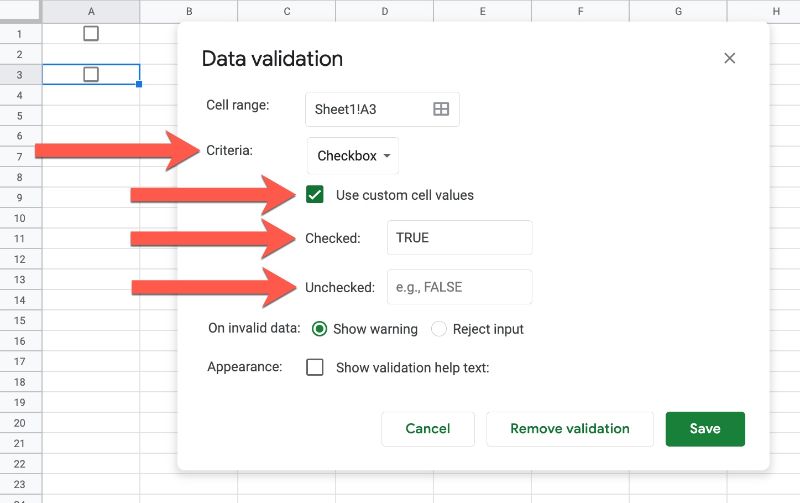
Add a checkbox to cell B1 through the Data menu: Data > Data validation
Under Criteria, select the checkbox.
Then select “Use custom cell values”
Set the TRUE value to be TRUE.
Set the FALSE value to be a blank cell (ignore the e.g. FALSE suggestion in the box already).
Step 2: Add More Checkboxes
Copy and paste this custom values checkbox into cells B2 and B3.
Step 3: Add Array Literal Formulas
In cell A1, add the following formula:
=IFERROR(IF(OR(B2,B3),{"Choice 1",""},),"Choice 1")This IF formula, in cell A1, looks at the checkbox values of B2 and B3 (i.e. the checkboxes on different rows). If either of them is checked then it sets the checkbox on this row to a blank value, set by the array literal part of the formula.
However, if neither of the other checkboxes in B2 and B3 is checked (i.e. neither of them are TRUE), then the IF formula gives an error.
In this case, the IFERROR function outputs a single string “Choice 1” and doesn’t interfere with the checkbox. The user is then free to select the checkbox if they wish.
In A2:
=IFERROR(IF(OR(B1,B3),{"Choice 2",""},),"Choice 2")And then in A3:
=IFERROR(IF(OR(B1,B2),{"Choice 3",""},),"Choice 3")Bingo!
With these formulas, you can only select a single checkbox at a time.
Step 4: Adding A Helper Prompt (Optional)
As mentioned, the main drawback with this method is that you have to uncheck the selected checkbox before you can select another one.
Since this is unintuitive behavior, it’s probably helpful to include a hint for your users.
In column C, you can add a set of simple IF formulas to do this.
E.g. in cell C1, add:
=IF(B1,"<-- uncheck before checking others",)And in cell C2:
=IF(B2,"<-- uncheck before checking others",)And finally, in cell C3:
=IF(B3,"<-- uncheck before checking others",)In practice, this looks like this:
Step 5: Extending To Larger Ranges
This simple example only considered 3 checkboxes, but you could include as many as you want.
You need to ensure that the checkboxes all have the custom values set up as shown above.
Then you need to include all the checkboxes except the current row in your OR condition. For example, if you have 10 checkboxes and you’re on row 5, then your OR condition needs to check if the checkboxes in rows 1 – 4 or rows 6 – 10 are checked.
Mimic Radio Buttons Template
Click here to open a view-only copy >>
Feel free to make a copy: File > Make a copy
If you can’t access the template, it might be because of your organization’s Google Workspace settings. If you right-click the link and open it in an Incognito window you’ll be able to see it.
You can omit the OR and IFERROR functions if you concatenate the inputs. For example, IF(B2&B3,{“Choice 1,””},”Choice 1″)
I like it. Thanks for sharing, Richard!