The IFERROR function in Google Sheets is a useful function to have in your Google Sheets toolbox. And it’s easy to learn.
In this tutorial you’ll learn how it works and see common use cases.
There are three principal uses for the IFERROR function:
- Replacing error values with a fallback value
- Catching errors and replacing default error messages with custom error messages
- In Array Formulas
IFERROR Function Syntax
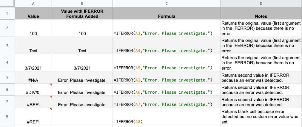
=IFERROR(value, [value_if_error])It takes two arguments.
The first argument is some value that you want to check for errors (see here for different types of errors in Google Sheets).
The second argument, which is optional, is the value you want to show if an error is detected. If this argument is omitted then a blank value is returned instead of an error.
When there is no error, the original value (set by the first value) is shown.
Let’s see an example of an IFERROR formula.
Suppose you have this formula in cell B1:
=IFERROR(A1,0)This formula checks the value of cell A1.
If cell A1 does not contain an error (e.g. it has a value like 10, or the word “Ben” or a date etc.) then it just returns that value.
However, if it detects an error in that cell (e.g. #N/A or #REF! etc.) then it returns the value 0.
IFERROR function example template
Click here to open a view-only copy >>
Feel free to make a copy: File > Make a copy…
If you can’t access the template, it might be because of your organization’s Google Workspace settings. If you click the link and open it in an Incognito window you’ll be able to see it.
Using The IFERROR Function To “Fix” Errors In Data
Suppose you have a column of calculated values in your Google Sheet, based off data elsewhere in the Sheet perhaps.
You want to change any errors to 0 (or whatever value you want) so that the column doesn’t contain any errors like #NA(). The #NA() error prevents you calculating a total for that column for example.
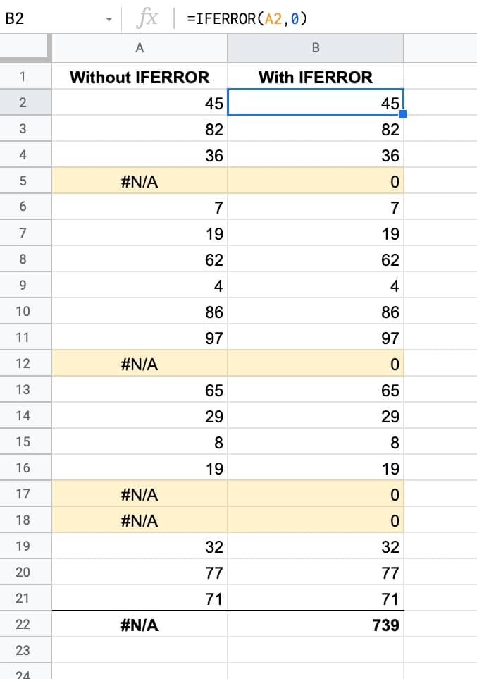
The formula in column B of this example is:
=IFERROR(A2,0)As you can see, the SUM function only calculates a total for column B where we replaced the #N/A errors with 0’s.
Using The IFERROR Function With Nested Formulas
Another common use case for IFERROR is as a wrapper around existing formulas that might output an error.
For example, if you’re using a VLOOKUP function and the search value is not found, it’ll return a #N/A error, which you may not want in your dataset.
Use IFERROR in front of the VLOOKUP and you can specify a custom error message e.g. “Search value not found”.
In this example we’re using VLOOKUP to search for a name in another table and return the property type that person lives in. In this case “Mr Ben Collins” was not found in the dataset. Compare columns B and C to see the different outputs with or without the IFERROR:
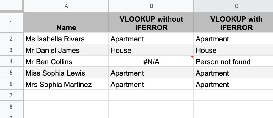
The formula in column C is:
=IFERROR( VLOOKUP( A2 , data!$B$1:$H$21 , 2 , false ), "Person not found" )Using the IFERROR Function With Array Formulas in Google Sheets
The IFERROR is useful when working with Array Formulas in Google Sheets.
Consider this Array Formula in cell B2:
=ArrayFormula(IF(A2:A <> "",A2:A * 100,IFERROR(1/0)))It works by looking down column A and wherever there’s a value in column A, it will multiple it by 100 and put the answer in column B.
Where cells in column A are empty, it returns a blank cell in column B.
The 1/0 gives a #DIV/0! error. The IFERROR(1/0) returns a blank cell.
It’s superior to just using a blank string "" because formulas will count the empty strings "", e.g. COUNTA() will count the blank cells if you use “” but not if you use IFERROR(1/0). In other words, it gives you a truly blank cell.
It’s the type of Array Formula commonly used in combination with Google Form data, where the calculations will be automatically calculated as new Form data arrives.
You can also read about it in the Google documentation.
So helpful! Been searching for a fix to this with subtotals and countifs for hours but this is the answer. Thank you 🙂
You’re welcome!