IF Function in Google Sheets

The IF function in Google Sheets is used to make decisions with your data. It’s from the Logical family of functions in Google Sheets.

In this tutorial, you’ll see how to use IF formulas in Google Sheets to make decisions with your data.

What does the IF Function do?

At its heart, the IF function is a test that evaluates to a true or false value with a defined behavior if the outcome is true and a different behavior when the outcome is false.

Let’s see an example.

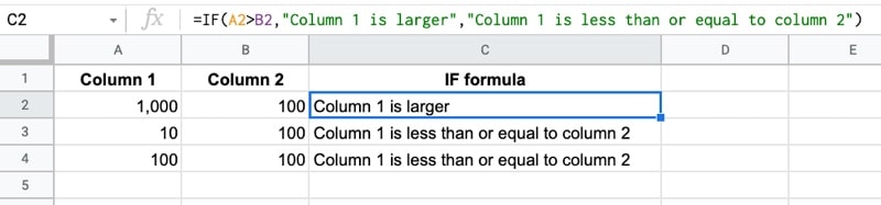
Suppose you have two columns of numbers in A and B and you want to compare each row to see which column has the larger number.

You would use the IF function in Google Sheets to do this!

Inside the IF formula, the first expression A2 > B2 checks whether the value in cell A2 is greater than the value in cell B2.

The outcome of this test is either a TRUE or a FALSE value.

The IF function requires a TRUE or FALSE value for this first argument.

Next up, you specify what you want to happen when the result is true. In this example the output of the function in the cell is “Column 1 is larger”

The final argument is the value you want to show if the result is false. In this example, that means the number in column A was smaller (or equal to) the value in column B. In this case, the output of the function is “Column 1 is less than or equal to column 2”.

IF Function in Google Sheets: Syntax

You might hear it referred to as an IF function, an IF formula or even an IF statement, but they all mean the same thing.

It takes 3 arguments:

logical_expression

An expression that gives a TRUE or FALSE answer, or a cell that contains a TRUE or FALSE value.

value_if_true

The value displayed by the IF function if the logical expression has the TRUE value.

value_if_false

The value displayed by the IF function if the logical expression has the FALSE value.

IF function template

Click here to open a view-only copy >>

Feel free to make a copy: File > Make a copy…

If you can’t access the template, it might be because of your organization’s Google Workspace settings. If you click the link and open in an Incognito window you’ll be able to see it.

The IF function is also covered in the Day 2 lesson of my free Advanced Formulas 30 Day Challenge course.

You can also read about it in the Google documentation.

Calculations with the IF Function in Google Sheets

IF functions can be combined with other functions to perform calculations on values above a certain threshold for example.

When the logical expression is true, do this calculation, otherwise leave the value as it is.

Perhaps your business has a performance bonus structure that pays out a 20% bonus above a certain threshold of client revenue. Use an IF statement to determine if the threshold has been met and then put the calculation in the true field:

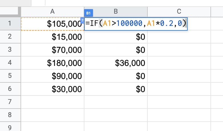
Using The IF Formula for Classification

Another example use case for the IF function is to classify items.

For example, you might want to segment your customers into long-term customers and new customers, based on whether they’ve been a client for 12 months or longer.

Suppose column A was a column containing the number of months a client has been with you, the following IF formula would classify them into long-term or new clients:

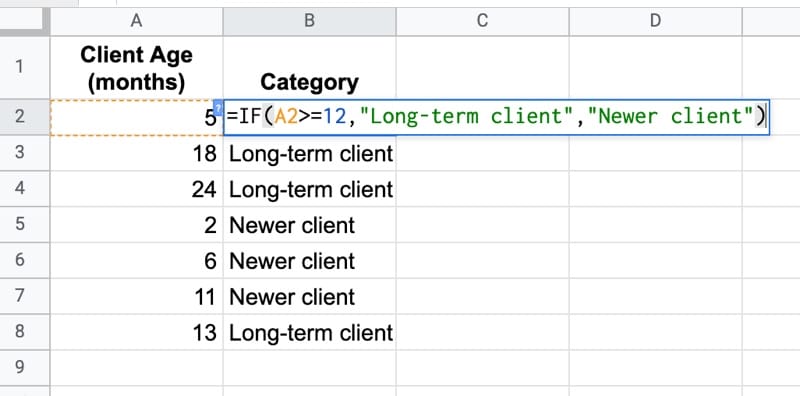
This kind of segmentation is useful in lots of different ways.

It lets you compare the retention and churn metrics of the two groups. You can run different marketing campaigns to different segments of your data. Or, maybe you just want to send a “Thank you, you’re awesome!” card to your long-term clients.

Nested IF Formula in Google Sheets

Sometimes one IF function alone isn’t enough.

Inside the TRUE or the FALSE arguments you can nest another IF function.

It looks complex but if you apply the onion method for working with formulas and work in layers, you’ll see it’s not difficult.

Working from the outside in, it checks if the value is greater than 50. If that is true, then the formula is done and it displays “Greater than 50”.

But if that’s false, it must mean the value is either less than 50 or equal to 50, so we use a second, nested IF to check for that:

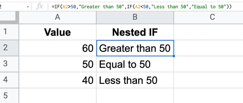
If your nested IF formulas get too complicated, you might want to try the SWITCH function.

IF Formulas and Checkboxes

Combining checkboxes with IF formulas is a powerful and versatile technique to use in your Sheets.

Checkboxes are actually just TRUE or FALSE values in disguise!

With a checkbox in cell A2, it can only ever have a TRUE or FALSE value. So it can be plugged into the IF function’s first argument directly!

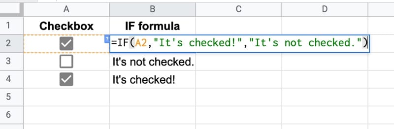
This sort of logic is useful in many settings, for example a dashboard where you want to show/hide additional context for specific numbers or charts.

Direct TRUE or FALSE Input

In the example above, you had a formula already in column A that contained a TRUE or FALSE value.

Since the first argument of the IF statement is looking for a TRUE of FALSE, you only need to reference that cell directly without testing for TRUE / FALSE.

Your IF formula would look like this:

There is NO need to test for TRUE or FALSE again. So you should not see an IF function like this:

In fact, you should never see an “= TRUE” or “= FALSE” in an IF statement because they’re redundant.

Replace numerical IF formulas with MIN or MAX functions

Suppose you have a column of values that you want to cap at a certain level, so that everything above a threshold value, e.g. 200, gets set to that value.

Most of us would approach this by writing an IF formula that checks whether the value is above 200 and then set it to 200 if TRUE, or the actual value if FALSE, like so:

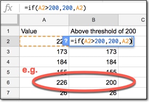
However, you can replace the whole IF function with a much more succinct MIN function, which chooses the value 200 if the actual value is larger, since 200 is the minimum:

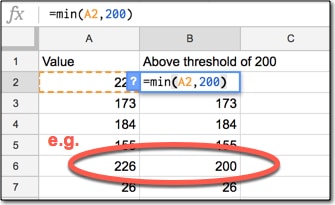
Similarly, we can use the MAX function to replace IF statements when we’re looking at a threshold on the low side.

It’s good practice to write efficient formulas because it’s quicker and you’re less likely to make mistakes.