INDIRECT Function in Google Sheets

The INDIRECT function in Google Sheets is used to convert text strings into valid cell or range references.

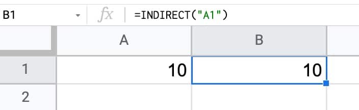
For example, the INDIRECT function will convert the text string “A1” into the cell reference A1. The formula is:

which is equivalent to this formula:

It gives the answer 10 in the following example because that’s the value in cell A1:

INDIRECT Function in Google Sheets: Syntax

It takes two arguments:

1. cell_reference_as_string
2. [is_A1_notation]

Here is what they mean:

cell_reference_as_string

The first argument is a text string that represents a cell or range reference, e.g.:

It can also point to a cell containing a range reference, as shown here:

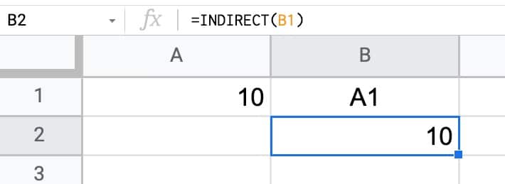
The value in cell B1 is the text value “A1”.

When the INDIRECT points to B1, it picks up this string reference and then converts it to an actual cell reference.

[is_A1_notation]

This second argument is an optional argument that is either TRUE or FALSE.

• If you set it to TRUE, the INDIRECT function to use familiar A1 style notation (e.g. A1, B2:D15, G1:M1000)
• Setting this argument to FALSE forces the INDIRECT function to use the uncommon R1C1 notation (see below)

If you omit this argument, and your INDIRECT just has a single argument like the example at the top of this page, it defaults to A1 notation as if you had used a TRUE argument.

I’ve never seen a formula with this second argument set to FALSE in the wild. So you can almost certainly ignore this argument and just use the INDIRECT function with a single input.

Aside On R1C1 Notation

R1C1 notation describes a cell or range reference using a row number and column number.

R1C1 is an absolute reference to the cell at position (1,1) in your Sheet, i.e. A1 in regular notation.

The reference with square brackets – R[1]C[1] – is a relative R1C1 reference meaning the cell 1 row down and 1 column to the right of the current cell, wherever that is in your worksheet.

Here’s an example of the INDIRECT using the R1C1 notation:

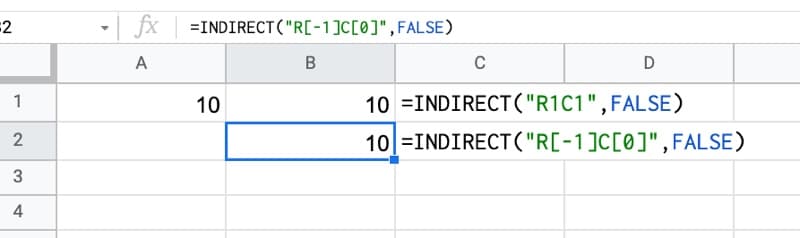
Both formulas have FALSE as the last argument of the INDIRECT function, so they’re using R1C1 notation.

The first has the absolute notation – “R1C1” – so it points to cell A1, the cell at Row 1 and Column 1 in your Sheet.

The second – “R[-1]C[0]” – is a relative reference telling the INDIRECT function to go back one row (i.e. the row above, going from row 2 to row 1) and stay in the same column (because the C value is 0).

This is equivalent to the formula:

R1C1 notation can also reference ranges by joining two cell references with a “:” colon, similar to how ranges are referenced in A1 notation, e.g.:

INDIRECT function template

Click here to open a view-only copy >>

Feel free to make a copy: File > Make a copy…

If you can’t access the template, it might be because of your organization’s Google Workspace settings. If you click the link and open it in an Incognito window you’ll be able to see it.

The INDIRECT function is also covered in the Day 22 lesson of my free Advanced Formulas 30 Day Challenge course.

You can also read about it in the Google documentation.

Using The INDIRECT Function To Work With Multiple Sheets

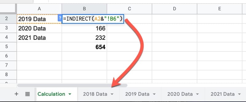
Suppose you have multiple sheets in you Google Sheets file, each with a similar structure. For example, it could be that you have transaction data per year, each in their own sheets: 2018 Data, 2019 Data, 2020 Data, 2021 Data

If you want to perform a calculation across all four sheets at once (e.g. a grand total), you have to click into each sheet from a formula and it’s rather tedious, especially if you have lots of sheets.

By using the INDIRECT function, you can build the formula with strings to save having to click on each tab.

With a list of sheet names in column A, use this INDIRECT formula in column B to access values from each sheet without needing to click across:

Drag this formula down the column and it will return the value in cell B6 of each sheet:

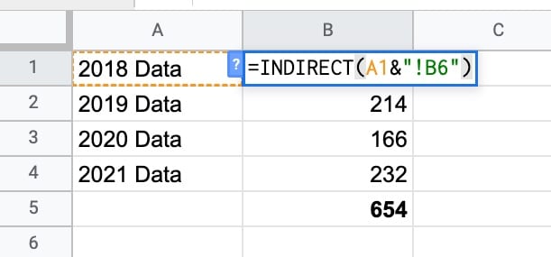
The first formula in cell B2 returns the value from cell B6 of the “2018 Data” sheet:

VLOOKUP + INDIRECT Formula in Google Sheets

This is another example of how to use the INDIRECT function to work with multiple sheets.

By combining the VLOOKUP function and INDIRECT functions, you can lookup data from different sheets based on a user input.

It requires you to have consistently named tabs in your Google Sheet, e.g. something like Data 2018, Data 2019, Data 2020, Data 2021

Create a Google Sheets drop down menu to let the user select one of these sheet names and then use the INDIRECT function to convert the text string into a valid range reference which becomes your lookup table.

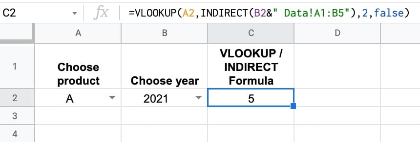
Using The INDIRECT Function To Create Vectors

NOTE: These methods have largely been replaced by the simpler, more elegant SEQUENCE function which can easily generate row or column vectors. However, you may still see the INDIRECT version in online forums or older resources, hence why I’m sharing here.

As you progress in your spreadsheet career, you’ll start to work more frequently with arrays of data rather than single values. One thing you’ll find yourself doing fairly often is needing to create a numbered list.

For example, you might want to sort data on the fly but need some way to get back to the original order. By using a combination of a column vector and array literals {…} you can build this inside the formula without having to add a helper column to your data.

Vectors crop up in other complex formulas too, like this text reverser, unpivot or even advanced sparklines like this clock or this visualize value experiment.

The INDIRECT function can be combined with the ROW function to create column vectors, or combined with the COLUMN function to create row vectors (yes, I realize that sounds strange, but you’ll see what I mean below).

This formula creates a vector from 1 to 10 running down a column:

This formula creates a vector from 1 to 10 running across a row:

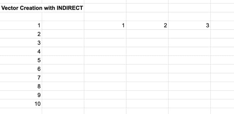
The formula can be generalized to create vectors of variable length. One example might be measuring the length of a text string in cell A1 and creating a vector matching that length.

This particular technique as part of a formula to reverse text in Google Sheets (again the newer SEQUENCE function could make this more succinct).

Other Advanced INDIRECT Techniques

The INDIRECT function can also be used to build dynamic named ranges in Google Sheets.

Read all about dynamic named ranges in Google Sheets here.