Unpivot in Google Sheets is a method to turn “wide” tables into “tall” tables, which are more convenient for analysis.
Suppose we have a wide table like this:
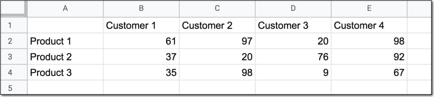
Wide data like this is good for the Google Sheets chart tool but it’s not ideal for creating pivot tables or doing analysis. The main reason is that data is captured in the column headings, which prevents you using it in pivot tables for analyis.
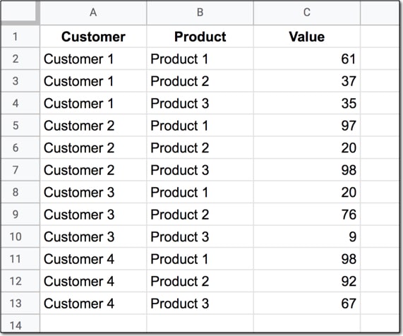
So we want to transform this data — unpivot it — into the tall format that is the way databases store data:
But how do we unpivot our data like that?
It turns out it’s quite hard.
It’s harder than going the other direction, turning tall data into wide data tables, which we can do with a pivot table.
This article looks at how to do it using formulas so if you’re ready for some complex formulas, let’s dive in…
Unpivot in Google Sheets
We’ll use the wide dataset shown in the first image at the top of this post.
The output of our formulas should look like the second image in this post.
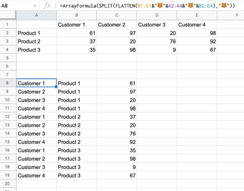
In other words, we need to create 16 rows to account for the different pairings of Customer and Product, e.g. Customer 1 + Product 1, Customer 1 + Product 2, etc. all the way up to Customer 4 + Product 4.
Of course, we’ll employ the Onion Method to understand these formulas.
Template
Click here to open the Unpivot in Google Sheets template
Feel free to make your own copy (File > Make a copy…).
(If you can’t open the file, it’s likely because your G Suite account prohibits opening files from external sources. Talk to your G Suite administrator or try opening the file in an incognito browser.)
Step 1: Combine The Data
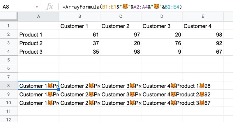
Use an array formula like this to combine the column headings (Customer 1, Customer 2, etc.) with the row headings (Product 1, Product 2, Product 3, etc.) and the data.
It’s crucial to add a special character between these sections of the dataset though, so we can split them up later on. I’ve used the fox emoji (because, why not?) but you can use whatever you like, provided it’s unique and doesn’t occur anywhere in the dataset.
=ArrayFormula(B1:E1&"🦊"&A2:A4&"🦊"&B2:E4)The output of this formula is:
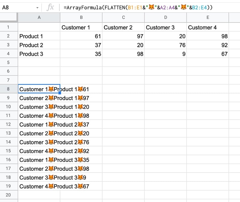
Step 2: Flatten The Data
Before the introduction of the FLATTEN function, this step was much, much harder, involving lots of weird formulas.
Thankfully the FLATTEN function does away with all of that and simply stacks all of the columns in the range on top of each other. So in this example, our combined data turns into a single column.
=ArrayFormula(FLATTEN(B1:E1&"🦊"&A2:A4&"🦊"&B2:E4))The result is:
Step 3: Split The Data Into Columns
The final step is to split this new tall column into separate columns for each data type. You can see now why we needed to include the fox emoji so that we have a unique character to split the data on.
Wrap the formula from step 2 with the SPLIT function and set the delimiter to “🦊”:
=ArrayFormula(SPLIT(FLATTEN(B1:E1&"🦊"&A2:A4&"🦊"&B2:E4),"🦊"))This splits the data into the tall data format we want. All that’s left is to add the correct column headings.
Unpivot With Apps Script
You can also use Google Apps Script to unpivot data, as shown in this example from the first answer of this Stack Overflow post.
Further Reading
For more information on the shape of datasets, have a read of Spreadsheet Thinking vs. Database Thinking.
There is a fifth solution.
I was looking for a solution to this very problem several months ago and after digging through forums for a couple of hours I found a custom function creatively named ‘UNPIVOT’ I no longer remember what forum led me to it but I found what appears to be the source:
https://gist.github.com/philippchistyakov/57390ec98dcaea4502fabc5a32242b3a
I use it on a daily basis and it’s delightful.
Enjoy!
Hi. This looks quite interesting. I tried to use it on the same example but couldn’t make it work. I get a message indicating “no data”: throw new Error(‘no data’); (line 21).
Is there anything I’m missing? I don’t have much experience with GAS so sorry if this is a silly question. Thank you!
Solved it myself! Now I understand. Thank you so much for all this info. Really useful!
How did you solve this?
Right, this is my exact problem… If I find the solutions I will post it.
So… it’s because I didn’t understand it being a custom function and you have to use it in the sheet where you want it to work. Data being the array you want to use.
The original link for the function is on stack exchange and includes an example.
https://stackoverflow.com/a/43681525
Yes! It was on StackExchange. Good call.
Power query of excel does this unpivot in a ziffy with a single click.
Yes, it was my solution as well
Helmanfrowsays, that custom formula is awesome!!!
Thanks, Ben, for your blog post about this advanced, but pretty important topic!
I was actually going to make a comment how I wish googlesheets had a melt() / unpivot() function (like python pandas) so that there’d be no need for all these nested ArrayFormula / Split / Flatten functions, but it’s great that there is already something circulating on github. Thank you for sharing this fifth solution!
This sheet gives single cell formula ( without using script) to unpivot a matrix by using FLATTEN function.
http://tiny.cc/unpivot
Honestly speaking I don’t think it can be further simplified.
Thanx a ton to Mr Prasanth for introducing FLATTEN function in his blog ( https://infoinspired.com/google-docs/spreadsheet/flatten-function-in-google-sheets/ )
Wow, very cool, S k srivastava! Thanks for sharing and to Pransanth for finding and documenting the FLATTEN function. I was not aware of that one!
Thanx. I modified it a bit. Now it can handle even more than one fixed column.
Is it possible to skip the empty cells? So for example skip Row1, Col2 in the result?
Prashanth did not find the flatten function. It was found by a user on the Google Sheets Community forums. This link is the discovery on 3/16/20.
https://support.google.com/docs/thread/33715001?hl=en
I modified the formula to Solution 4 a little bit to handle product names with double spaces (for example: Product Name). The original formula would trim those double spaces into single space.
=ArrayFormula(SPLIT(REGEXREPLACE(TRANSPOSE(SPLIT(TRANSPOSE(QUERY(TRANSPOSE(QUERY(TRANSPOSE(IF(Sheet1!B2:Z””, Sheet1!A2:A&”
I added more columns and was having issues if not all columns had data in them. To fix this I modified solution 4 to put a space with each fish when creating the formula, as I found when there was an empty column of data (so you ended up with two fish next to each other before the final split), it would miss a column, but adding a space in (but not as the split identifier) made it work, and the columns all line up. Just need to add an additional trim to get rid of the extra spaces after the final split.
=ArrayFormula(
{
“Product”,”Other”,”one more”,”Customer”,”Value”;
QUERY(
iferror(trim(split(TRIM(TRANSPOSE(SPLIT(TRANSPOSE(QUERY(TRANSPOSE(QUERY(TRANSPOSE(IF(Sheet1!D2:AA””, Sheet1!A2:A&”
Actually, now i have an issue with the above, where the final trim is somehow turning all Numeric and date fields into “text” and gsheets doesn’t seem to want to let me format them as numbers? Any suggestions appreciated.
Hi Ben, thank you for sharing the undocumented FLATTEN() method; it was exactly what I was looking for!
This seems overly complicated to me. You can use & to do most of the work, like this:
=arrayformula(split(flatten(arrayformula(A2:A4 &”
Yes, agreed! But the article was written before I was aware of the flatten function 😉
This is great, but I have a question. What if your table has blank values, and in your “unpivoted” table you don’t want those rows to show up? Is there any way to remove them by altering this formula? For example, in the above table, B2 has a blank value (not 0, just blank). In my results, I do not want to see a row for Customer 1 – Product 1 since the Value would be blank.
I had this same issue. The bigger problem is that blanks in your original/raw data will cause the range returned by split/flatten trick to shift (definitely not what we want in that case)
Would be interested to hear from Ben on his advised approach to handling this. (please let us know, Ben )
Ben – there must be a way to tell Google sheets/array functions to not “skip” blank cells, right? (seems to be the default behavior)
But for now I stumbled on a solution to wrap any ranges you reference with a condition that checks if cell is blank and returns a single apostrophe character if it is (I first tried having it return “”, like is often used in these situations), but that just creates the same problem we’re trying to avoid.
Example:
IF(B2:E4″”,B2:E4,”‘”)
You could also use 0 if it makes sense for your data set. In my case using 0 wasn’t appropriate b/c its an actual valid/possible value and I needed something to mean “no data”.
IF(B2:E4″”,B2:E4, 0)
Or of course you can replace zeros with blanks in your original/raw data, again if zero makes sense for your data set
CORRECTION:
IF(B2:E4″”, B2:E4,”‘”)
(Somehow syntax got messed up when I copied/pasted into the comment)
Ahh, looks like characters get changed when I enter the comment…
IF condition should check B2:E4 is NOT equal to an empty string (double quotes)
Great Solution, thanks for sharing.
Thanks, Ben! I never thought this could be done without a lot of manual work!
Small suggestion: perhaps you could update the article to include at the top the suggestion to use FLATTEN. I had to scroll down the stackoverflow link you included to find this beautifully simple solution that was all I needed:
=ARRAYFORMULA(SPLIT(FLATTEN(A2:A12&”//”&B1:F1&”//”&B2:F12),”//”))
Hi
This is useful but the issue I am facing is I have data spread horizontally need to convert them vertically not able to find a solution anywhere used transpose function but suppose horizontal data is in row 1 2 and three it gave me output in 3 different columns A , B and C I want that to be in one single column also not getting if there is a space in between how to exclude that please help me out Ben .
Hi, I was looking for something similar, however I have a more complicated data than this.
Instead of just column A, I have Columns A to I, and then instead of just a single column of data, I have 4 columns each to append to data in A:I.
Data gathered from forms with various sections.
Can you help me with the same?
I needed to handle this for a situation where the number of rows changes. I found this article
https://medium.com/@nnamdi.okafor/getting-the-last-row-with-values-on-google-sheets-10aa6aaf855f
and used the second function – 1st didn’t work and I was too busy to troubleshoot.
Result for vertical ranges then becomes, for example (instead of A2:A):
indirect(“A2:A”&sum(max(arrayformula(if(A1:A “”,row(A:A),”” )))))
This has worked amazingly!
Thanks Ben. I have until now worked with an unpivot script (I think I saw it mentioned in the comments) but it’s not a live function, i.e it has to be run every time the data changes. This function of yours doesn’t, which means I can now automate what has been a manual step in so many processes.
We can achieve this with the pivot function itself just need to fix the column names in the pivot.
See here: https://drive.google.com/file/d/1VzgEI90Ixhd_VBLbTqLDYgR9sksBBqZP/view
Fantastic!!! Thanks for help=]
Hi,
Excellent formula, thank you.
Is it possible to filter automatically? I am unpivotting several columns and rows but in some cases the values are empty. This creates rows that are not needed.
Can a filter be added so that empty cells on a specific column are not included as a row?
Thanks
Hy,
These is awesome, but i have a little problem. I have a sheet where I test these and it works but when I put it into the work sheet it gives me #Error! I don’t undersand what I’m doing wrong.
Please help
This was a helpful tip.
One thing I ran into when dealing with empty columns was the split function behaves weirdly with an emoji. I ended up having to use this split to ensure things lined up:
split(,””,false,false)
If the second argument is true, then the emoji is treated as two characters (it seems) and you end up with an extra column. If the second column is true (the default), you end with your data misaligned.
The split function in the unpivot above doesn’t handle blank cells well, resulting in the data ending up misaligned.
The below split works better and will ensure blank cells are treated the same as cells with data:
SPLIT(,””,false, false)
Note the third parameter is important or Google Sheets will introduce a blank column when using an emoji as the delimiter [I reported it as a bug].
Thank you, this was super helpful and helped me simplify my formulas a ton, which is a huge deal when working with 15,000 rows of data!!
You’re welcome! cheers!