 💡 Sponsored Link
Grow your business with secure, collaborative tools. Try Google Workspace free for 14 days and enjoy all the latest and greatest Sheets features!
Starting from $6 per user / month.
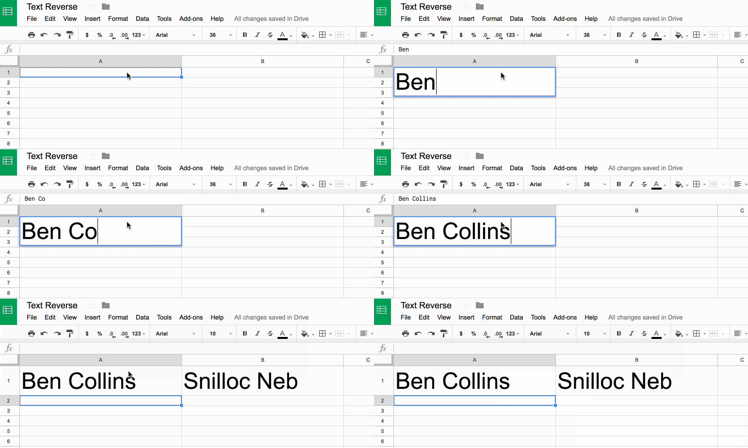
In this example, you’ll see how to reverse text in Google Sheets.
To start, enter some text into cell A1 and the formula in cell B1, to reverse the order of the text:

Reverse Text In Google Sheets
What’s the formula?
=ArrayFormula(IFERROR(PROPER(CONCATENATE(MID(A1,LEN(A1)-ROW(INDIRECT("1:"&LEN(A1)))+1,1))),""))It’s a beast! See below for a detailed breakdown of how it works.
It might be useful if you wanted to find the last character in a string, or the last occurrence of a character using the FIND() function.
Here’s an alternative, which reverses the capitalization too (submitted by Michael D over email – thanks!):
=JOIN("",ARRAYFORMULA(MID(A1,LEN(A1)-ROW(INDIRECT("1:"&LEN(A1)))+1,1)))Can I see an example worksheet?
How does this formula work?
Basically we make an array of numbers corresponding to how many letters are in the original text string. Then we reverse that, so the array shows the largest number first. Then we extract each letter at that position (so the largest number will extract the last letter, the second largest will extract the second-to-last letter, etc., all the way to the smallest number extracting the first letter). Then we concatenate these individual letters.
Easy! Err…
The only way to really understand this formula is to break it down, starting from the inner functions and building back out.
Assuming we have the text string “Abc” in cell A1, then let’s build the formula up in cell B1, step-by-step:
Step 1:
Use the LEN function to calculate the length of the text string and turn it into a range string with “1:”&LEN(A1)
Use the INDIRECT function to turn this string range reference into a valid range reference.
Finally wrap with ROW to convert into a row number list.
=ROW(INDIRECT("1:"&LEN(A1)))which outputs a result of 1 in cell B1.
Step 2:
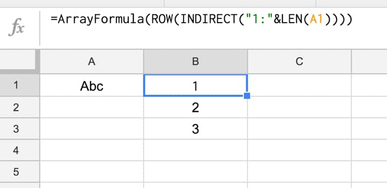
Turn the formula into an array formula, by hitting Ctrl + Shift + Enter, or Cmd + Shift + Enter (on a Mac), to the formula above. This will add the ArrayFormula wrapper around the formula:
=ArrayFormula(ROW(INDIRECT("1:"&LEN(A1))))This outputs 1 in cell B1, 2 in cell B2 and 3 in cell B3:

Step 3:
Reverse the output, so 3 is in cell B1, 2 in B2 and 1 in B3, by subtracting from the length of the text in A1 and adding 1 to avoid 0:
=ArrayFormula(LEN(A1)-ROW(INDIRECT("1:"&LEN(A1))) + 1)Step 4:
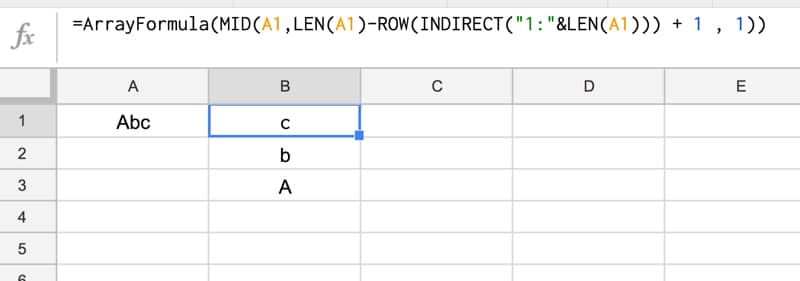
Use the MID formula to now extract the letters at position 3 (“c”), position 2 (“b”) and position 1 (“A”) and display in cells B1:B3:
=ArrayFormula(MID(A1,LEN(A1)-ROW(INDIRECT("1:"&LEN(A1))) + 1 , 1))so your output is now:

Step 5:
Concatenate so that all the individual outputs are combined into a single cell:
=ArrayFormula(CONCATENATE(MID(A1,LEN(A1)-ROW(INDIRECT("1:"&LEN(A1))) + 1 , 1)))
Step 6 (optional):
The string is essentially reversed now, so we could stop here.
However, you can use the PROPER function to capitalize the first letters of each word only, for a true reverse effect:
=ArrayFormula(PROPER(CONCATENATE(MID(A1,LEN(A1)-ROW(INDIRECT("1:"&LEN(A1))) + 1 , 1))))Step 7 (optional):
Last step is to add in an IFERROR function to avoid an unsightly error message if the input cell (A1) is blank:
=ArrayFormula(IFERROR(PROPER(CONCATENATE(MID(A1,LEN(A1)-ROW(INDIRECT("1:"&LEN(A1)))+1,1))),""))Final output:
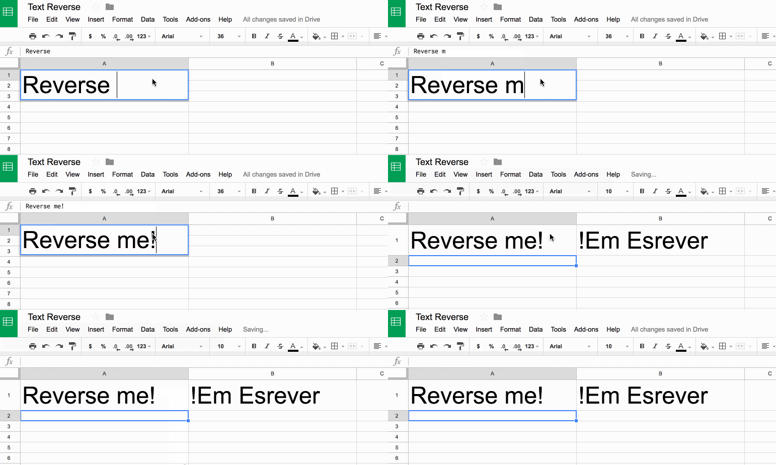
Here’s the formula in action again:

Further Reading
You might also like this article on Using Text Rotation to Create Custom Table Headers in Google Sheets.
Hi there!
First of all, thank you for your awesome website – my spreadsheet skills must have gone up ten-fold just as a result of being able to look at the many formula examples you’ve given across the site – Bravo!
I work in a genomics laboratory and had a related problem to the ‘reversing text’ one described – I needed to ‘reverse complement’ a few thousand short DNA sequences (we need to do this as the base-pairs that form in DNA are between strands which antiparallel – they are running in opposite directions to each other). I’m not a Bioinformatician (they would do this using Perl/Python), so I came looking for inspiration here. In the end, I came up with the following which I leave here just in case anyone is interested (e.g. for a DNA sequence in A2):
=CONCATENATE(SWITCH(ARRAYFORMULA(MID(A2,LEN(A2)-SEQUENCE(LEN(A2))+1,1)),"A","T","G","C","T","A","C","G"))Note that this will throw up an error if the source sequence contains any letters other than A, T, G or C, or any lower-case characters.
As another non-bioinformaticist biologist, thank you for this formula!
Hey I found another shorter formula that (as far as I know) does the same thing. I used:
=JOIN("",ArrayFormula(MID(A1,LEN(A1)-SEQUENCE(1,LEN(A1))+1,1)))For what it’s worth, this version definitely seems better as it avoids the volatile INDIRECT function.
This works great, thanks for creating it. Apparently even google AI (Genimi) thinks it is not possible in google sheets.Lol!