Using Text Rotation to Create Custom Table Headers in Google Sheets

The text rotation feature in Google Sheets rotates text in a cell, so it can be angled in any direction.

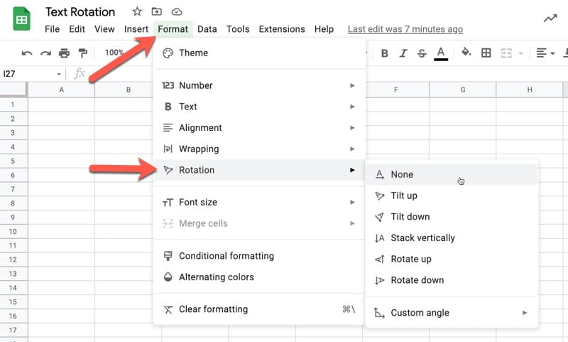
Find text rotation under the menu: Format > Rotation

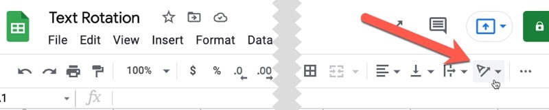
It can also be accessed by a button on the far right side of the toolbar:

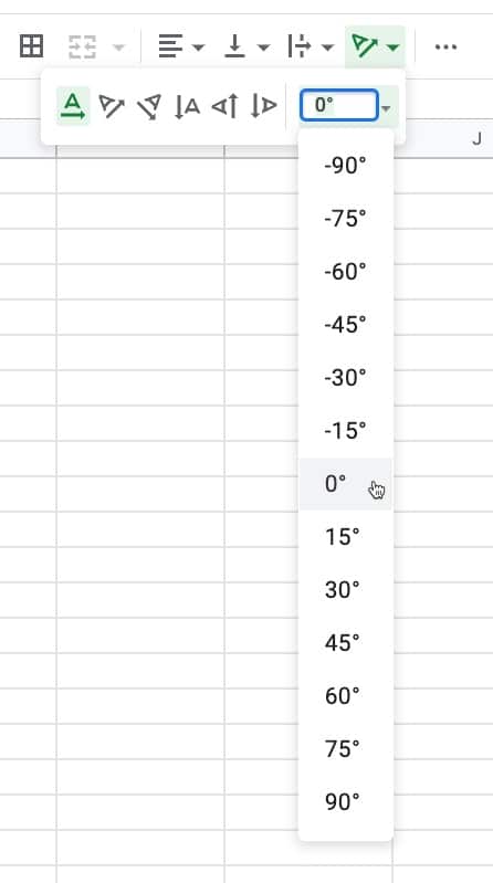
There are six preset modes as well as a custom angle option:

Text Rotation Options

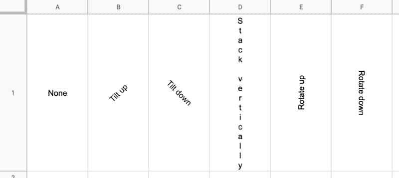
• None – no text rotation
• Tilt up – angle text upwards at 45°
• Tilt down – angle text downwards at 45°
• Stack vertically – stack the letters on top of each other vertically
• Rotate up – rotate the text 90° up
• Rotate down – rotate the text 90° down
• Custom angle – select an angle or type a custom angle

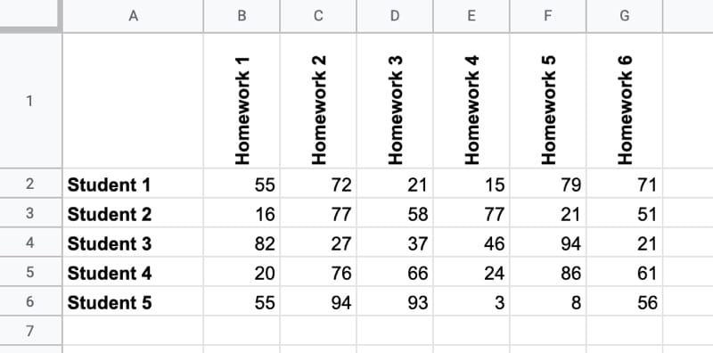
Example 1: Text Rotation Headings

The most straightforward use case is to rotate headers upwards to save space and avoid wide columns:

Example 2: Text Rotation Sidebar

Add flourishes to your dashboards in Google Sheets by using text rotation to create branded sidebars:

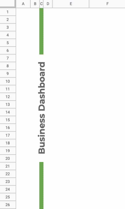
This is achieved by merging cells, rotating text upwards inside the merged cell, adding a background color to column C, and then making B, C, and D narrow.

Example 3: Text Rotation to Subdivide Cell

This example was prompted by a question from a reader:

How do I make a diagonal line to split a cell, so that I can enter text into two triangular subdivisions?

Although you can’t split a cell explicitly, you can use rotated text to achieve this effect.

This solution featured as tip 38 of my Google Sheets newsletter.

Here’s an example showing a diagonal line to separate the row and column heading labels in a single cell:

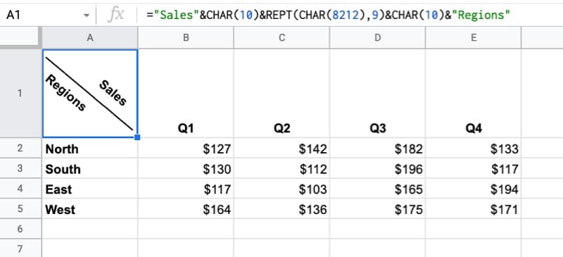
To achieve this, use the CHAR function, the REPT function, and rotate the text.

The formula is:

How does this work?

This function creates a line break:

CHAR(10) 

And this one creates the em-dash character:

CHAR(8212) 

Finally, the REPT function repeats the CHAR function 9 times, i.e. it creates 9 em-dash characters, which gives the appearance of the line:

REPT(CHAR(8212),9)

To finish, center align the cell and then rotate the text downwards using a custom angle around -40°.

Caveat

You should only use this method for formatting and not for analysis.

Use it for presentation tables only, because it makes dataset column headings a mess for analysis work, like pivot tables or charts. Generally, labels in column A need their own column heading.

Alternative Way To Subdivide A Cell

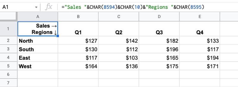
Here, the formula is:

This formula uses three different CHAR functions to add context and force a line break.

• CHAR(8594) produces the right arrow
• CHAR(10) produces a carriage return (new line)
• CHAR(8595) produces a down arrow

It makes the table much easier to interpret and reduces the chance of a user misreading the data.

This example is taken from the customer analysis section of my Data Analysis with Google Sheets course.

More Table Formatting Tips

For more tips on formatting tables in Google Sheets, check out this post: How To Make a Table in Google Sheets, and Make It Look Great

Text Rotation Template

Click here to open a view-only copy >>

Feel free to make a copy: File > Make a copy…

However, if you can’t access the template, it might be because of your organization’s Google Workspace settings.

In this case, right-click the link to open it in an Incognito window to view it.