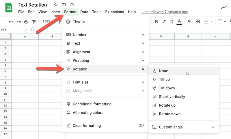
The text rotation feature in Google Sheets rotates text in a cell, so it can be angled in any direction.
Find text rotation under the menu: Format > Rotation
Continue reading Using Text Rotation to Create Custom Table Headers in Google Sheets
Educator and Google Developer Expert. Helping you navigate the world of spreadsheets & AI.
The text rotation feature in Google Sheets rotates text in a cell, so it can be angled in any direction.
Find text rotation under the menu: Format > Rotation
Continue reading Using Text Rotation to Create Custom Table Headers in Google Sheets
In this post, we’ll look at how to wrap text in Google Sheets so that long strings fit inside cells and can be read easily.
Select a range of data and go to the menu: Format > Wrapping > Wrap
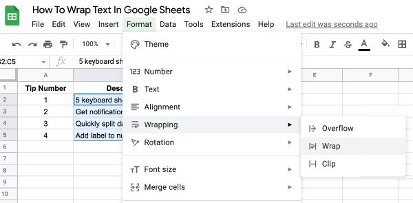
Next to the wrap text option, you’ll find the clip option (show on one line and don’t allow any overflow) and overflow option (show on one line and allow to spill into adjacent cells).
Google Sheets custom number format rules are used to specify special formatting rules for numbers.
These custom rules control how numbers are displayed in your Sheet, without changing the number itself. They’re a visual layer added on top of the number. It’s a powerful technique to use because you can combine visual effects without altering your data.
Sheets already has many built-in formats (e.g. accounting, scientific, currency etc.) but you may want to go beyond and create a unique format for your situation.
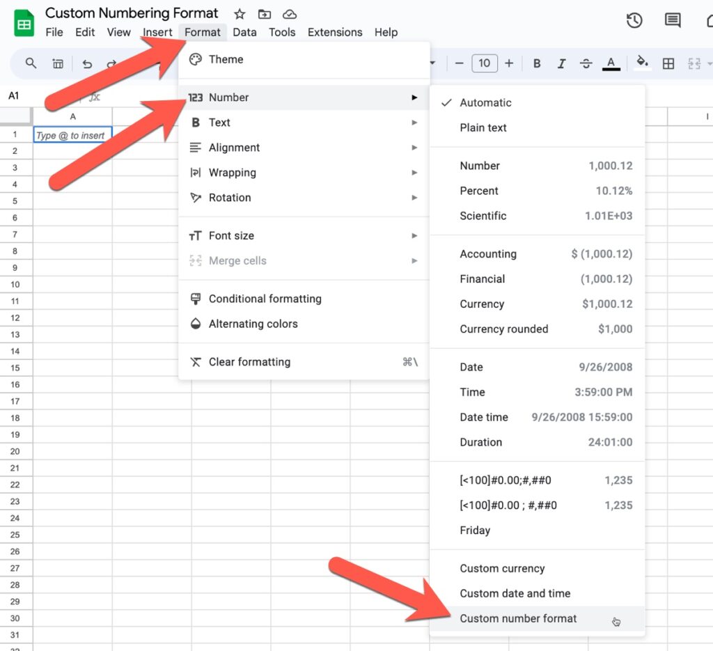
Access custom number formats through the menu:
Format > Number > Custom number format
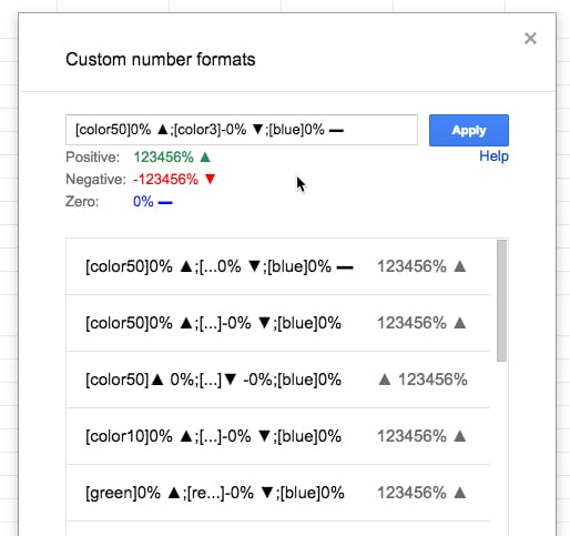
The custom number format editor window looks like this:
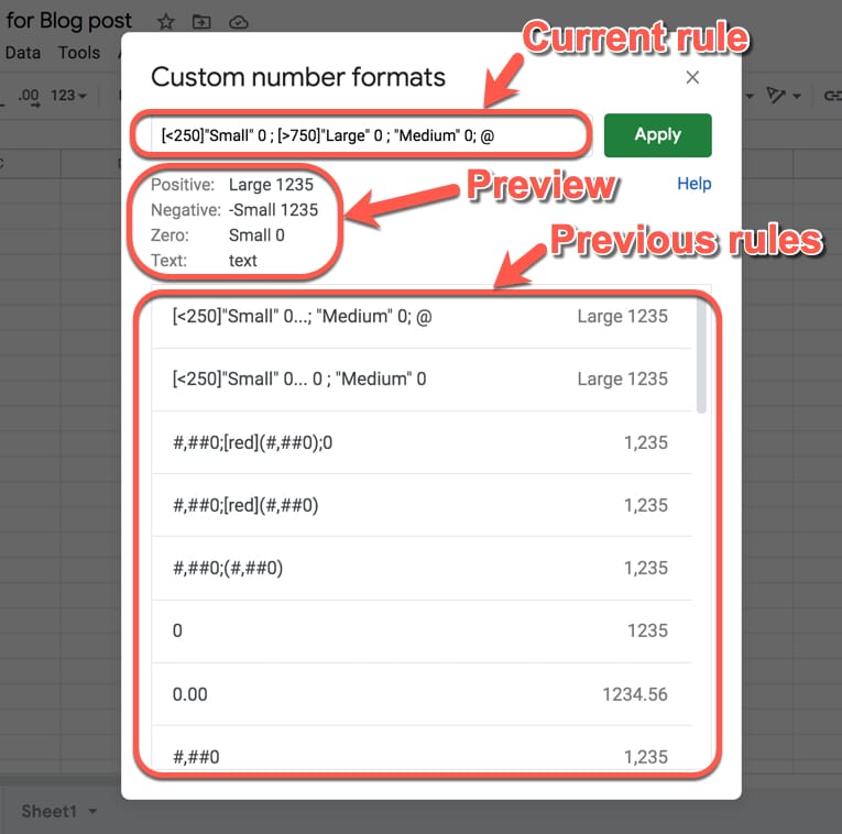
You type your rule in the top box and hit “Apply” to apply it to the cell or range you highlighted.
Under the input box you’ll see a preview of what the rule will do. It gives you a useful and pretty accurate indication of what your numbers will look like with this rule applied.
Previous rules are shown under the preview pane. You can click to restore and reuse any of these.
You have four “rules” to play with, which are entered in the following order and separated by a semi-colon:
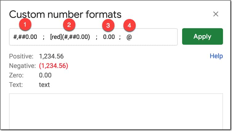
#,##0.00 ; [red](#,##0.00) ; 0.00 ; “some text “@
The first rule, which comes before the first semi-colon (;), tells Google Sheets how to display positive numbers.
#,##0.00 ; [red](#,##0.00) ; 0.00 ; “some text “@
The second rule, which comes between the first and second semi-colons, tells Google Sheets how to display negative numbers.
#,##0.00 ; [red](#,##0.00) ; 0.00 ; “some text “@
The third rule, which comes between the second and third semi-colons, tells Google Sheets how to display zero values.
| Rule | Before | After |
|---|---|---|
0;0;"Zero" |
0 | Zero |
#,##0.00 ; [red](#,##0.00) ; 0.00 ; “some text “@
The fourth rule, which comes after the third semi-colon, tells Google Sheets how to display text values.
No, you don’t have to specify them all everytime.
If you only specify one rule then it’s applied to all values.
If you specify a positive and negative rule only, any zero value takes on the positive value format.
Here are some examples of single- and multi-rule formats:
| Rule | Positive | Negative | Zero | Text |
|---|---|---|---|---|
0 |
1 | -1 | 0 | text |
0;(0) |
1 | (1) | 0 | text |
[red]0 |
1 | -1 | 0 | text |
0;[red]-0 |
1 | -1 | 0 | text |
0;[red]-0;[blue]0;[green]@ |
1 | -1 | 0 | text |
Zero (0) is used to force the display of a digit or zero, when the number has fewer digits than shown in the format rule. Use the zero digit rule (0) to force numbers to be a certain length and show leading zero(s).
For example:
| Rule | Before | After |
|---|---|---|
0.00 |
1.5 | 1.50 |
00000 |
721 | 00721 |
The pound sign (#) is a placeholder for optional digits. If your value has fewer digits than # symbols in the format rule, the extra # won’t display anything.
| Rule | Before | After |
|---|---|---|
#### |
15 | 15 |
#### |
1589 | 1589 |
#.## |
1.5 | 1.5 |
The comma (,) is used to add thousand separators to your format rule. The rule #,##0 will work for thousands and millions numbers.
| Rule | Before | After |
|---|---|---|
#,##0 |
1495 | 1,495 |
#,##0.00 |
1234567.89 | 1,234,567.89 |
The period (.) is used to show a decimal point. When you include the period in your format rule, the decimal point will always show, regardless of whether there are any values after the decimal.
| Rule | Before | After |
|---|---|---|
0. |
10 | 10. |
0. |
10.1 | 10. |
0.00 |
10 | 10.00 |
If you add thousand separators but don’t specify a format after the comma (e.g. 0,) then the hundreds will be chopped off the number. Combine this with a “k” or “K” to indicate the thousands and you have a nice way to showcase abbreviated numbers. To achieve this with millions, you need to specify two commas.
| Rule | Before | After |
|---|---|---|
0.0, |
2500 | 2.5 |
0,"k" |
2500 | 3k |
0.0,"k" |
2500 | 2.5k |
0.0,,"M" |
1234567 | 1.2M |
Brackets can be added to the negative number rule to change the format from -100 to (100), which is often seen in accounting and financial scenarios.
| Rule | Before | After |
|---|---|---|
0;(0) |
-100 | (100) |
The asterisk (*) is used to repeat digits in your format rule. The character that follows after the asterisk is repeated to fill the width of the cell.
In the following example, the dash is repeated to fill the width of the cell in Google Sheets:
| Rule | Before | After |
|---|---|---|
*-0 |
100 | ——————100 |
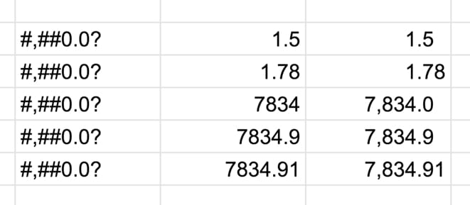
The question mark (?) is used to align values correctly by adding necessary space, even when the number of digits don’t match.
See this example:
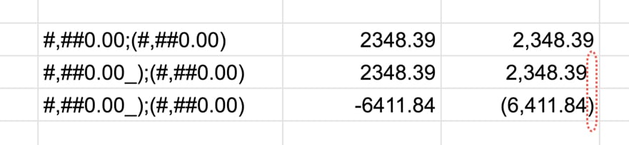
The underscore (_) also adds space to your number formats.
In this case, the character that follows the underscore determines the size of the space to add (but is not shown). So this rule allows you to add precise amounts of space.
For example #,##0.00_);(#,##0.00) adds a space after the positive sign that is the width of one bracket, so that the decimal point lines up with the negative numbers with brackets.
You can see this clearly in the following image, where the first line does NOT have the spacing but the second line does. The red highlight has been added to show the result of the spacing:
Suppose you want to actually show a pound sign in your format. If you simply add it into your format rule, then Sheets will interpret it as a placeholder for optional digits (see above).
To actually show the pound sign, precede it with a backslash (\) to ensure it shows.
This applies to any of the other special characters too.
| Rule | Before | After |
|---|---|---|
#0 |
10 | 10 |
\#0 |
10 | #10 |
The At symbol (@) is used as a placeholder for text, which means don’t change the text entered.
| Rule | Before | After |
|---|---|---|
0;0;0;"Special text value!" |
Some text | Special text value! |
0;0;0;@ |
Some text | Some text |
The forward slash (/) is used to denote fractions.
For example, the rule # ?/? will show numbers as fractions:
| Rule | Before | After |
|---|---|---|
# ?/? |
2.3333333333 | 2 1/3 |
The percent sign (%) is used to format values as %. As with the other rules, you first specify the digits and then use the % sign to change to a percent e.g. 0.00%
| Rule | Before | After |
|---|---|---|
0.00% |
0.2829 | 28.29% |
For very large (or very small) numbers, use the exponent format rule to show them more compactly.
The rule is: number * E+n, in which E (the exponent) multiplies the preceding number by 10 to the nth power.
Let’s see an example:
| Rule | Before | After |
|---|---|---|
0.00E+00 |
23976986 | 2.40E+07 |
Adding conditions inside of square brackets replaces the default positive, negative and zero rules with conditional expressions.
For example:
| Rule | Before | After |
|---|---|---|
[<100]"Small" ; [>500]"Large" ; "Medium" |
50 | Small |
[<100]"Small" ; [>500]"Large" ; "Medium" |
300 | Medium |
[<100]"Small" ; [>500]"Large" ; "Medium" |
800 | Large |
Meta instructions for conditional rules from the Google Sheets API documentation.
Add colors to your rules with square brackets [ ].
There are 8 named colors you can use:
[black], [white], [red], [green], [blue], [yellow], [magenta], [cyan]
To get more colors, use the 2-digit color codes written:
[Color1], [Color2], [Color3], ..., [Color56]
For full rundown of the color palette for these 56 colors, click here.
| Rule | Before | After |
|---|---|---|
0;[red](0) |
-100 | (100) |
Here’s another example of using Google Sheets custom number format rules with colors: How To Make a Table in Google Sheets, and Make It Look Great
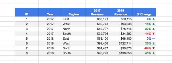
where the rule is:
Meta instructions for color rules from the Google Sheets API documentation.
Turn any 11 digit number into a formatted telephone number with the zero digit rule and dashes:
| Rule | Before | After |
|---|---|---|
0 000-000-0000 |
18004567891 | 1 800-456-7891 |
Use conditional rules to pluralize words. Remember, these are still numbers under the hood so you can still do arithmetic with them. The formatting portion (“day” or “days”) is just added as a layer on top.
| Rule | Before | After |
|---|---|---|
[=1]0" day"; 0" days" |
1 | 1 day |
[=1]0" day"; 0" days" |
2 | 2 days |
[=1]0" day"; 0" days" |
100 | 100 days |
Use conditionals to classify numbers directly:
| Rule | Before | After |
|---|---|---|
[<250]"Small"* 0 ; [>750]"Large"* 0 ; "Medium"* 0 |
70 | Small 70 |
[<250]"Small"* 0 ; [>750]"Large"* 0 ; "Medium"* 0 |
656 | Medium 656 |
[<250]"Small"* 0 ; [>750]"Large"* 0 ; "Medium"* 0 |
923 | Large 923 |
Note: these are still numbers under the hood, so you can do arithmetic with them. Moreso, the “Small”, “Medium” and “Large” only exist in the format layer and cannot be accessed in formulas. For example, you can’t use a COUNTIF to count all the values with “Large”. To do that, you need to actually change the value so the word “Large” is in the cell, or add a helper column.
The “* ” part of the rule adds space between the word and the number so that it fills out the full width of the cell.
Add color scales to the conditional example:
| Rule | Before | After |
|---|---|---|
[color44][<250]"Small"* 0;[color46][>750]"Large"* 0;[color45]"Medium"* 0 |
70 | Small 70 |
[color44][<250]"Small"* 0;[color46][>750]"Large"* 0;[color45]"Medium"* 0 |
656 | Medium 656 |
[color44][<250]"Small"* 0;[color46][>750]"Large"* 0;[color45]"Medium"* 0 |
923 | Large 923 |
Combine conditionals with emojis to turn numbers into a emoji-scale, like this temperature example:
| Rule | Before | After |
|---|---|---|
[>90]🔥🔥🔥;[>50]🔥;❄️;"No data" |
37 | ❄️ |
[>90]🔥🔥🔥;[>50]🔥;❄️;"No data" |
75 | 🔥 |
[>90]🔥🔥🔥;[>50]🔥;❄️;"No data" |
110 | 🔥🔥🔥 |
[>90]🔥🔥🔥;[>50]🔥;❄️;"No data" |
N/a | “No data” |
How To Add Subscript and Superscript In Google Sheets
Google documentation on how to format numbers in Sheets.
Custom Number Format Builder for Google Sheets and Excel.
Questions? Comments? Have you used custom number formats? Seen any interesting examples? Leave a comment below.