
Google Sheets custom number format rules are used to specify special formatting rules for numbers.
These custom rules control how numbers are displayed in your Sheet, without changing the number itself. They’re a visual layer added on top of the number. It’s a powerful technique to use because you can combine visual effects without altering your data.
Sheets already has many built-in formats (e.g. accounting, scientific, currency etc.) but you may want to go beyond and create a unique format for your situation.
Google Sheets Custom Number Format Usage
Access custom number formats through the menu:
Format > Number > Custom number format
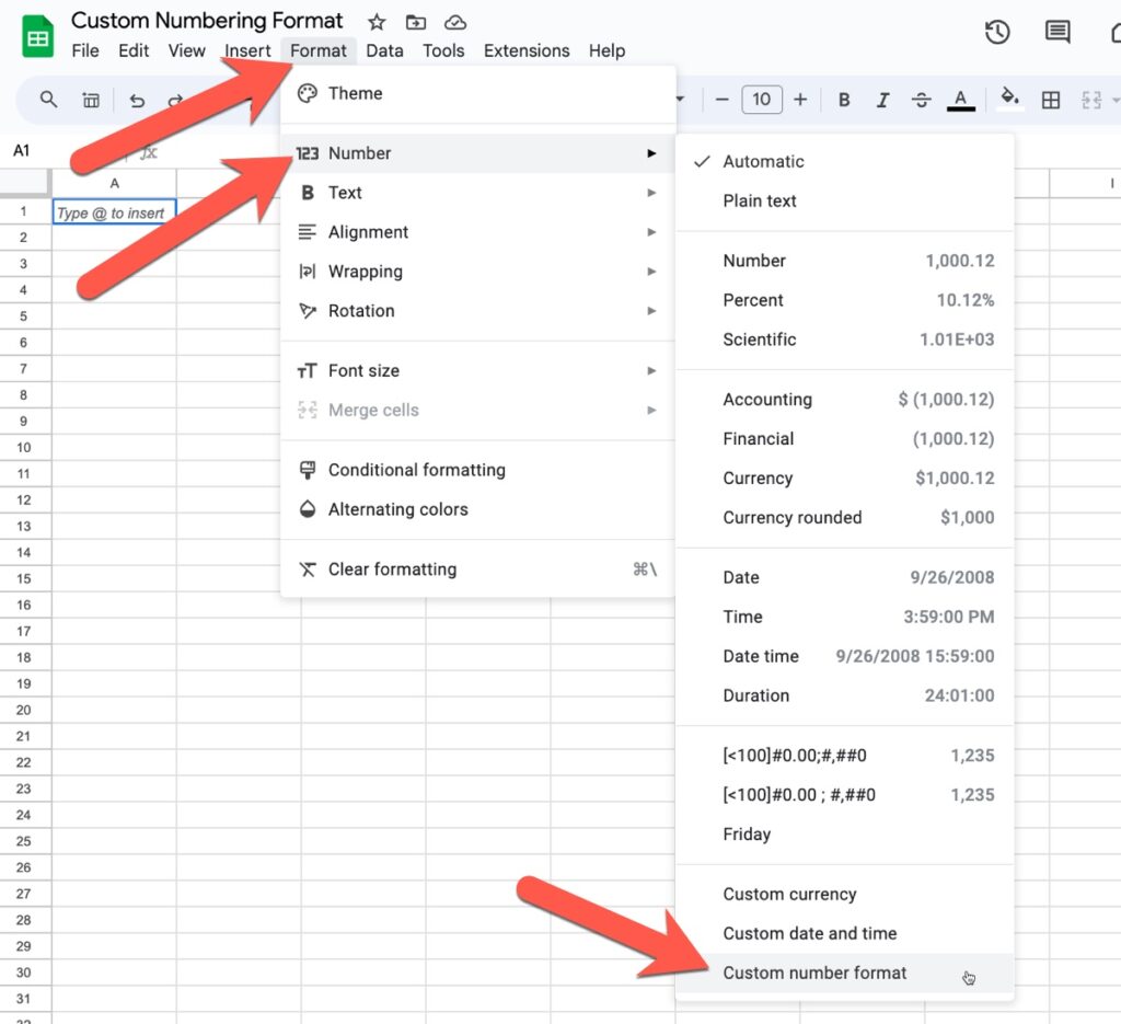
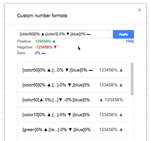
The custom number format editor window looks like this:
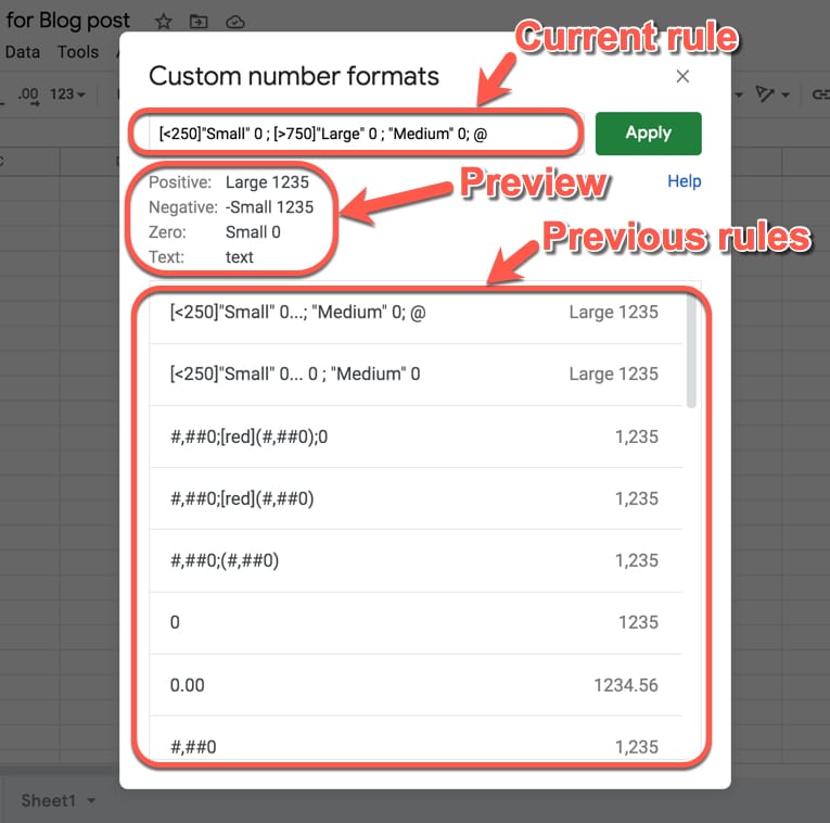
You type your rule in the top box and hit “Apply” to apply it to the cell or range you highlighted.
Under the input box you’ll see a preview of what the rule will do. It gives you a useful and pretty accurate indication of what your numbers will look like with this rule applied.
Previous rules are shown under the preview pane. You can click to restore and reuse any of these.
Google Sheets Custom Number Format Structure
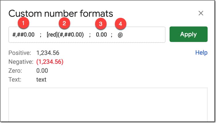
You have four “rules” to play with, which are entered in the following order and separated by a semi-colon:
- Format for positive numbers
- Format for negative numbers
- Format for zeros
- Format for text
1. Format for positive numbers
#,##0.00 ; [red](#,##0.00) ; 0.00 ; “some text “@
The first rule, which comes before the first semi-colon (;), tells Google Sheets how to display positive numbers.
2. Format for negative numbers
#,##0.00 ; [red](#,##0.00) ; 0.00 ; “some text “@
The second rule, which comes between the first and second semi-colons, tells Google Sheets how to display negative numbers.
3. Format for zeros
#,##0.00 ; [red](#,##0.00) ; 0.00 ; “some text “@
The third rule, which comes between the second and third semi-colons, tells Google Sheets how to display zero values.
| Rule | Before | After |
|---|---|---|
0;0;"Zero" |
0 | Zero |
4. Format for text
#,##0.00 ; [red](#,##0.00) ; 0.00 ; “some text “@
The fourth rule, which comes after the third semi-colon, tells Google Sheets how to display text values.
Do You Have To Use All Four Rules?
No, you don’t have to specify them all everytime.
If you only specify one rule then it’s applied to all values.
If you specify a positive and negative rule only, any zero value takes on the positive value format.
Here are some examples of single- and multi-rule formats:
| Rule | Positive | Negative | Zero | Text |
|---|---|---|---|---|
0 |
1 | -1 | 0 | text |
0;(0) |
1 | (1) | 0 | text |
[red]0 |
1 | -1 | 0 | text |
0;[red]-0 |
1 | -1 | 0 | text |
0;[red]-0;[blue]0;[green]@ |
1 | -1 | 0 | text |
Google Sheets Custom Number Format Rules
Zero Digit Rule (0)
Zero (0) is used to force the display of a digit or zero, when the number has fewer digits than shown in the format rule. Use the zero digit rule (0) to force numbers to be a certain length and show leading zero(s).
For example:
| Rule | Before | After |
|---|---|---|
0.00 |
1.5 | 1.50 |
00000 |
721 | 00721 |
Pound Sign Rule (#)
The pound sign (#) is a placeholder for optional digits. If your value has fewer digits than # symbols in the format rule, the extra # won’t display anything.
| Rule | Before | After |
|---|---|---|
#### |
15 | 15 |
#### |
1589 | 1589 |
#.## |
1.5 | 1.5 |
Thousands Separator (,)
The comma (,) is used to add thousand separators to your format rule. The rule #,##0 will work for thousands and millions numbers.
| Rule | Before | After |
|---|---|---|
#,##0 |
1495 | 1,495 |
#,##0.00 |
1234567.89 | 1,234,567.89 |
Period (.)
The period (.) is used to show a decimal point. When you include the period in your format rule, the decimal point will always show, regardless of whether there are any values after the decimal.
| Rule | Before | After |
|---|---|---|
0. |
10 | 10. |
0. |
10.1 | 10. |
0.00 |
10 | 10.00 |
Thousands (k or K) or Millions (m or M)
If you add thousand separators but don’t specify a format after the comma (e.g. 0,) then the hundreds will be chopped off the number. Combine this with a “k” or “K” to indicate the thousands and you have a nice way to showcase abbreviated numbers. To achieve this with millions, you need to specify two commas.
| Rule | Before | After |
|---|---|---|
0.0, |
2500 | 2.5 |
0,"k" |
2500 | 3k |
0.0,"k" |
2500 | 2.5k |
0.0,,"M" |
1234567 | 1.2M |
Negative Number With Brackets ( )
Brackets can be added to the negative number rule to change the format from -100 to (100), which is often seen in accounting and financial scenarios.
| Rule | Before | After |
|---|---|---|
0;(0) |
-100 | (100) |
Asterisk (*)
The asterisk (*) is used to repeat digits in your format rule. The character that follows after the asterisk is repeated to fill the width of the cell.
In the following example, the dash is repeated to fill the width of the cell in Google Sheets:
| Rule | Before | After |
|---|---|---|
*-0 |
100 | ——————100 |
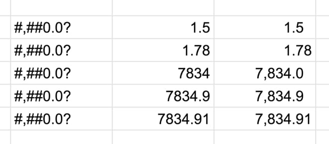
Question Mark (?)
The question mark (?) is used to align values correctly by adding necessary space, even when the number of digits don’t match.
See this example:
Underscore (_)
The underscore (_) also adds space to your number formats.
In this case, the character that follows the underscore determines the size of the space to add (but is not shown). So this rule allows you to add precise amounts of space.
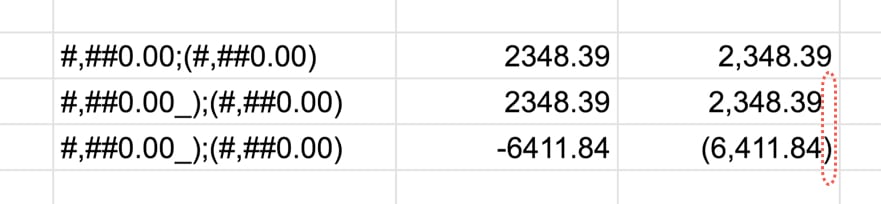
For example #,##0.00_);(#,##0.00) adds a space after the positive sign that is the width of one bracket, so that the decimal point lines up with the negative numbers with brackets.
You can see this clearly in the following image, where the first line does NOT have the spacing but the second line does. The red highlight has been added to show the result of the spacing:
Escape Character (\)
Suppose you want to actually show a pound sign in your format. If you simply add it into your format rule, then Sheets will interpret it as a placeholder for optional digits (see above).
To actually show the pound sign, precede it with a backslash (\) to ensure it shows.
This applies to any of the other special characters too.
| Rule | Before | After |
|---|---|---|
#0 |
10 | 10 |
\#0 |
10 | #10 |
At (@)
The At symbol (@) is used as a placeholder for text, which means don’t change the text entered.
| Rule | Before | After |
|---|---|---|
0;0;0;"Special text value!" |
Some text | Special text value! |
0;0;0;@ |
Some text | Some text |
Fraction (/)
The forward slash (/) is used to denote fractions.
For example, the rule # ?/? will show numbers as fractions:
| Rule | Before | After |
|---|---|---|
# ?/? |
2.3333333333 | 2 1/3 |
Percent (%)
The percent sign (%) is used to format values as %. As with the other rules, you first specify the digits and then use the % sign to change to a percent e.g. 0.00%
| Rule | Before | After |
|---|---|---|
0.00% |
0.2829 | 28.29% |
Exponent (E)
For very large (or very small) numbers, use the exponent format rule to show them more compactly.
The rule is: number * E+n, in which E (the exponent) multiplies the preceding number by 10 to the nth power.
Let’s see an example:
| Rule | Before | After |
|---|---|---|
0.00E+00 |
23976986 | 2.40E+07 |
Google Sheets Custom Number Format Conditional Rules
Adding conditions inside of square brackets replaces the default positive, negative and zero rules with conditional expressions.
For example:
| Rule | Before | After |
|---|---|---|
[<100]"Small" ; [>500]"Large" ; "Medium" |
50 | Small |
[<100]"Small" ; [>500]"Large" ; "Medium" |
300 | Medium |
[<100]"Small" ; [>500]"Large" ; "Medium" |
800 | Large |
Conditional Rules
- Conditions can only be specified in the first two rules
- The third rule is used as the format for everything else that doesn’t satisfy the first two conditions
- The fourth rule is always used for text, so cannot be used for conditional formatting
Meta instructions for conditional rules from the Google Sheets API documentation.
Colors In Google Sheets Custom Number Formats
Add colors to your rules with square brackets [ ].
There are 8 named colors you can use:
[black], [white], [red], [green], [blue], [yellow], [magenta], [cyan]
To get more colors, use the 2-digit color codes written:
[Color1], [Color2], [Color3], ..., [Color56]
For full rundown of the color palette for these 56 colors, click here.
Color Examples
| Rule | Before | After |
|---|---|---|
0;[red](0) |
-100 | (100) |
Here’s another example of using Google Sheets custom number format rules with colors: How To Make a Table in Google Sheets, and Make It Look Great
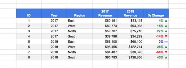
where the rule is:
Meta instructions for color rules from the Google Sheets API documentation.
Google Sheets Custom Number Format Examples
Telephone
Turn any 11 digit number into a formatted telephone number with the zero digit rule and dashes:
| Rule | Before | After |
|---|---|---|
0 000-000-0000 |
18004567891 | 1 800-456-7891 |
Plural
Use conditional rules to pluralize words. Remember, these are still numbers under the hood so you can still do arithmetic with them. The formatting portion (“day” or “days”) is just added as a layer on top.
| Rule | Before | After |
|---|---|---|
[=1]0" day"; 0" days" |
1 | 1 day |
[=1]0" day"; 0" days" |
2 | 2 days |
[=1]0" day"; 0" days" |
100 | 100 days |
Conditional
Use conditionals to classify numbers directly:
| Rule | Before | After |
|---|---|---|
[<250]"Small"* 0 ; [>750]"Large"* 0 ; "Medium"* 0 |
70 | Small 70 |
[<250]"Small"* 0 ; [>750]"Large"* 0 ; "Medium"* 0 |
656 | Medium 656 |
[<250]"Small"* 0 ; [>750]"Large"* 0 ; "Medium"* 0 |
923 | Large 923 |
Note: these are still numbers under the hood, so you can do arithmetic with them. Moreso, the “Small”, “Medium” and “Large” only exist in the format layer and cannot be accessed in formulas. For example, you can’t use a COUNTIF to count all the values with “Large”. To do that, you need to actually change the value so the word “Large” is in the cell, or add a helper column.
The “* ” part of the rule adds space between the word and the number so that it fills out the full width of the cell.
Conditional + Color
Add color scales to the conditional example:
| Rule | Before | After |
|---|---|---|
[color44][<250]"Small"* 0;[color46][>750]"Large"* 0;[color45]"Medium"* 0 |
70 | Small 70 |
[color44][<250]"Small"* 0;[color46][>750]"Large"* 0;[color45]"Medium"* 0 |
656 | Medium 656 |
[color44][<250]"Small"* 0;[color46][>750]"Large"* 0;[color45]"Medium"* 0 |
923 | Large 923 |
Temperature Example
Combine conditionals with emojis to turn numbers into a emoji-scale, like this temperature example:
| Rule | Before | After |
|---|---|---|
[>90]🔥🔥🔥;[>50]🔥;❄️;"No data" |
37 | ❄️ |
[>90]🔥🔥🔥;[>50]🔥;❄️;"No data" |
75 | 🔥 |
[>90]🔥🔥🔥;[>50]🔥;❄️;"No data" |
110 | 🔥🔥🔥 |
[>90]🔥🔥🔥;[>50]🔥;❄️;"No data" |
N/a | “No data” |
Other Resources
How To Add Subscript and Superscript In Google Sheets
Google documentation on how to format numbers in Sheets.
Custom Number Format Builder for Google Sheets and Excel.
Questions? Comments? Have you used custom number formats? Seen any interesting examples? Leave a comment below.
VERY informative! Thanks a lot – so nice to know.
Thanks, Chrilles!
Brilliant tutorial and reference – really helped me solve a tricky formatting problem on which I was stuck. Many thanks!
Hi Ben! I have a question regarding Custom Number Format with a space as a separator. I’m using:
– ### as a hundreds separator,
– # ### as a thousands separator,
– ### ### as a ten and hundred-thousand separator,
– ### ### ### as a millions separator.
There is a catch in my reports though, where a number could be 1 234 567 one day and 876 000 another. With custom format I mentioned above, it’s formatted correctly in first case, but wrong in second – it would look like ” 876 000″ (notice the space at first decimal). Is there any way how to resolve the problem, so it would look like “876 000” without a space with such formatting?
Thanks!
Miroslav
PS: Keep up good work, absolutely loving your articles by the way
Hi, Ben,
Like all your posts, this is really clear and useful. Apart from all the good stuff you explain, I’ve found the text option useful for data validation pulldowns. The interface doesn’t explain it, but here @ represents the text value in the cell, to which you can add what you like before and after.
Suppose you have a cell for the user to choose a day of the week to take off. You can always label that in an adjacent cell, but I prefer formatting the text as “Take “@”off.” That lets the cell display an unambiguous “Take Tuesday off.” while containing only the useful value “Tuesday”.
Another excellent resource. Thanks for compiling this!
I’ve been using custom number formats in Google Sheets for as long as Sheets has been around, and I just doubled my usable knowledge. A really great site!
Hi,
Thanks for posting this article.
I would like any number above 999,999.99 to be formatted as #,##0.00,,”M” then any number below 1,000,000.00 to be marked as $#,##0.00,K. Is there a way to do this in Google Sheets?
Thanks,
Ben
[<999950]0.0,"K";[<999950000]0.0,,"M";0.0,,,"B"
Can you please break this down?
Related question: is there any way to apply rounding based on the size of the number? e.g.
if A1 = 1,234,567 then apply =round(a1, -6)
if A1 = 234,567 then apply =round(a1, -5)
Hi,
I need you help to make a number short for Thousands”, “Lakhs” & “Crores”.
The currency rule:
0 to 99,999 ===> K
1,00,000 to 99,99,999 ==> L
1,00,00,000 + ==> C
Any guidance please.
Tried this but it dint work
[<99999]0.0,"K";[<9999999]0.0,,"L";0.0,,,"C"
Hi,
I want to do amount conversion into “Thousand”, “Lakhs” & “Crores”
Rule:
0 to 99,999 ==> “K”
1,00,000 to 99,99,999 ==> “L”
1,00,00,000 + ===> “C”.
I tried the below formula but it didn’t work
[<99999]0.0,"K";[<9999999]0.0,,"L";0.0,,,"C"
Please suggest what I am doing wrong
You’re probably looking for something like this:
[<999.950]0.0;[-999.950]0.0;[>-999950]0.0,”K”;0.0,,”M”
I haven’t found a way to do that with both positive and negative at the same time. Also it’s not expandable up to Billions, Trillions, etc. so I instead use this formula:
[>999.949]###.0E+00;[<-999.949]###.0E+00;0.0
This is much more expandable because it uses scientific notation for every three decimal places meaning:
0.9 = 0.9
9.9 = 9.9
99.9 = 99.9
999.9 = 999.9
9,999.9 = 9.9E+03
99,999.9 = 99.9E+03
999,999.9 = 999.9E+03
9,999,999.9 = 9.9E+06
etc.
This looks complicated, but because it's every third decimal place, you can read E+03 as thousand, E+06 as million etc. which is much easier than normal scientific notation or just keeping the big number in your spreadsheet. While the previous formula works for positive and negative numbers, though it doesn't work for large decimals. for that you have to use this:
[<.999950]###.0E+00;[-.999950]###.0E+00;[>-999.950]0.0;###.0E+00
This is probably more than you need, but I hope you find this helpful.
Hi Ben,
We have a table that is pulling via VLOOKUP from a selection of other tables based on a couple of dropdown cells at the top (with a fairly long IFS formula). Some of the source tables are “Impressions” #,### and some are “Spend” $#,###. Is there a way to conditionally format the numbers in the table to either match the format of the source data… changing as it also changes? Or make some kind of conditional format rule where if cell C5 is “Impressions” it formats D6:O39 as #,### and if C5 is “Spend” it formats D6:O30 as $#,###? I actually have that working on one document but one of my team members is building out a similar document for a different client and for some reason it isn’t happening. I have no idea if I did something special to make it work in the other document, I honestly don’t think I did, I think the numbers just followed the source and change back and forth magically. But for some reason the new document is NOT doing that and it is driving us mad trying to figure out how to tell it to do so.
Thanks so much for your help!
Ali
Same issue here! Haven’t found solution yet…
Hi,
I want to do amount conversion into “Thousand”, “Lakhs” & “Crores”
Rule:
0 to 99,999 ==> “K”
1,00,000 to 99,99,999 ==> “L”
1,00,00,000 + ===> “C”.
I tried the below formula but it didn’t work
[<99999]0.0,"K";[<9999999]0.0,,"L";0.0,,,"C"
Please suggest what I am doing wrong
Hey, did you find any solution to add lakhs and crores suffix in google finance sheet with custom number format help?
fairly new to google sheets. lets say i want to have a cell that i can enter a number , that number adds to another cell and then clears so i can enter another number. is this possible?
I need your to help to make a number from 123456789 to 12,34,56,789
Can you help me to convert 150000 to 1.5?
Is there a format that will turn
12.34567 into 12.34 (easy enough)
without also turning
12 into 12. (with an extraneous decimal point)
Yes!
In other words: I want integers to be left alone and not have a trailing period appended. Thank you!
Great question. I’d like to know as well .
No answer to this one, eh? Seems like a common need. Not a fixed but a maximum number of decimal places.
0.## is the idea, but nobody wants to see “12.”
Still looking for a solve to this one.
if i have 8.45456 = 8.4 and 6 = 6 (not 6. )
Please advise.
Hi there, thanks for the info!
I have a question. In Excel I use this custom format :
@ * “:”
What it does is, it put a “:” on the far right of the cells, regardless of the cells length, so there will always be a colon, and it will always be on the far right. Any way to do that in Sheets? I’ve been tinkering with it and got stumped lol.
Hello, I need this too, and I couldn’t find a solution.
were you able to find it? If you succeed, I would like you to share.
Or if there is someone who can help, please do not hesitate to support.
regards
Great info, really helpful. Just one thing I need help with. I need to format my google sheet to display spaces in between numbers I’m scanning in.
A scanned number will come in at 111122223333 but I need it to have spaces
eg. 1111 2222 3333
Thanks!
Hello,
Is there any format that allow 1 to become 1DR (not 1.0DR nor 1.DR) and 1.2 to become 1.2DR ?
I tried 0.0″DR” but 1 became 1.0DR
I tried #.#”DR” but 1 become 1.DR
In Excel it was quite easy to do that : put the format of the numbers as Standard”DR”
I’m lookin generate a 5 character count using 0-9 & A-Z
that will generate as a line/record is made.
0000A-
0001A-
0002A-
Number count would continue to 9999A- and then then the next letters of the alphabet would be used.
Could use numbers in one cell and letter in another and =A1&B1
But it would be amazing if it could populate from a formula on its own as a record is made as a counter.
very informative…
I have a question, what should i do, if i want to fix the number of digits in any cell? for e.g. I want to enter any mobile number in a cell have exactly 10 digits not more than 10 nor less than 10
I’m making a report to show whole numbers without decimals and dashes for zeros. However, google sheets show 0 instead of a dash for numbers between 0.1 and 0.4. Anything numbers above or equal to 0.5 will be round up as 1. I don’t want to use the round formula to round to whole numbers because the total will be off.
So I try to get around with the following formula but I don’t know how to present negative numbers in brackets.
[=1]#,##0; “-”
Please help! Thank you!
Sorry, part of the formula got cut off. I tried with this: [=1]#,##0;”-“
Hi JC,
Best I could get is with
[>=0.5]#,##0;[<=-0.5]#,##0;-When you use the conditionals, you have two conditions and then a default value option. It's slightly different to the positive;negative;zero;text of the regular custom number formats. So I couldn't find a way to replace the minus sign with the brackets when using these conditionals.
Hope this helps!
Ben
Hi Ben!
I’m using the positive/negative number formatting to track changes in a spreadsheet from one year to the next (in the simplest terms, cell A1=10, B1=15, C1 has a formula of B1-A1 with the aforementioned Custom Number Formatting, so that C1=+5).
However, in some cases, I do not have a value for B1, so I have written a formula that pulls A1 straight to C1 when a numerical value is not present in B1, but does the math when a value is there…=if(B1=”*”,A1,(B1-A1)). The formula is doing exactly what I want it to do, but the number formatting is applying the ‘+’ sign, which is not accurate. Is there a way to bypass the custom formatting based on the formula in the cell, so that I don’t have to manually disable the formatting in those cases?
Or is this a pipe dream…
I used the formula:
[<999950]0.00,"K"; [<999950000]0.00,,"M"
This changed 1,250 to 1.25K and 1,250,000 to 1.25M, which was what I wanted.
However, it also changed 250 to 0.25K, which was not a desired outcome.
I tried:
[<1000]0; [<999950]0.00,"K"; [<999950000]0.00,,"M"
and despite each section working on their own, and working in pairs, the three together is considered an "Invalid format".
I'd prefer to be able to apply this format to the whole document, rather than manually applying [<1000]0 where necessary.
Any advice/alternative formulas are welcome.
Hi Alexander,
As you’ve discovered you’re only allowed two logical tests, but you are allowed to use the 3rd position as the default value. So you can test for millions, then thousands, and then set the third value as the regular number, e.g.
[>999999]#,##0.000,,"M";[>999]0.00,"K";0Hope this helps.
Cheers,
Ben
How to add new line in custom number format. like
16 dec 2022
saturday
Thanks, very helpful
Hi Ben,
I’m wondering if it isn’t possible to create a custom number formatting, so that the numbers are displayed in the European way (without changing language settings)?
So I want to exchange comma with period:
(i.e. from 1,006,000.11 to 1.006.000,11)
Before I was successful with the date formatting – but with numbers I wasn’t able to do it; as I require, as it breaks the logic as soon I use the comma in custom number format.
Is there any way to show a set number of digits after a decimal point but to also show no decimal if the number is a perfect integer?
To rephrase:
Is there a format that hides the decimal point when displaying integer values?
Is it possible to see and edit the custom format for a given cell?
If I click on a cell and then click on the Custom Format menu item, I do not see the format formula for that cell. For example, I clicked on a cell that contains a number preceded by a plus sign (+) but the custom format dialog opened with the formula ‘0’ in it. Logically, this cannot be the current format.
I can see cells with more complicated formats and I don’t want to have to reverse engineer them in order to edit them.
Hello can you help me to make this number 321339308 to 3.21, on my sheet it shows like this 321,339,308, thank you
This is a very helpful, well-executed reference guide, which leads me to wonder why Google couldn’t have published a document like this, themselves.
Great article. Quick question: I assume it’s not possible for the conditions to be anything other than = or > or < tests, yes? I'm trying to apply a different format to all even numbers and can't work out how… (odd request i know, but i have my reasons)
I'm using [=2]-;[=0]-;0 to catch the first 2 even numbers, but i wanted a simple one that catches all even numbers, but [=iseven()]-;0 and things of that nature appear not to work…
Hi, thanks for your article!
I still have one problem:
I want 171,75 formatted as 171:45 h. (I want to display durations)
Thanks!
Interesting! I didn’t know how to do this for you, but I think this is a text value, not a number. The comma is not a thousands separator, so I think it is part of a text string. You need more than a format, you need an operation to replace the comma with a semicolon, and then append ” h” to show units. Is that right?
Great explanation, many thanks!
This is a fantastic guide that had to take many hours, research and skill to create. Usually such things have 487 ads polluting the experience. I don’t see any! Why did you produce this? Can we compensate you somehow?
Thanks, James! Best way to help me is to sign up for my weekly newsletter 🙂