How To Use The IMPORTRANGE Function In Google Sheets To Transfer Data From One Sheet To Another

Since Google Sheets are files in the cloud, not on your desktop, you can’t click on a cell in a different Sheets file to connect them.

Instead, you use the IMPORTRANGE function in Google Sheets to connect Google Sheet files and import data from one Sheet file into another.

Once set up, the function will automatically sync with the source data so that changes are reflected in the destination Sheet.

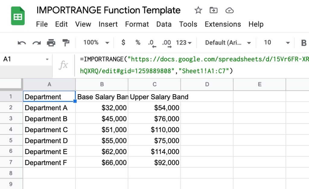
If you look closely, you’ll see a URL in the formula — the URL of the source Google Sheet file, where the data is being imported from.

How To Use The IMPORTRANGE Function In Google Sheets

For this example, suppose you have a dataset of department salaries in one Sheet that you want to import into a different Google Sheets file.

Step 1:

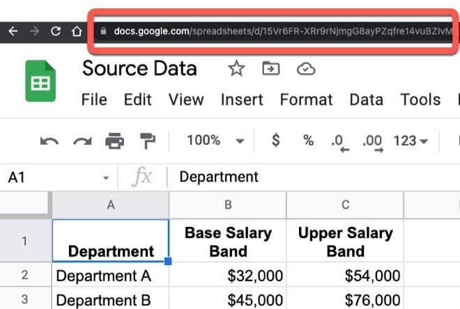
Copy the entire URL of the source Sheet, shown here in red:

Step 2:

In your destination Google Sheet, where you want to import this data, enter this formula with the URL from step 1 (the URL of your source Sheet):

Step 3:

Complete the formula by adding the sheet name and range reference, from the Source Sheet, of the data you want to import, e.g.:

Step 4:

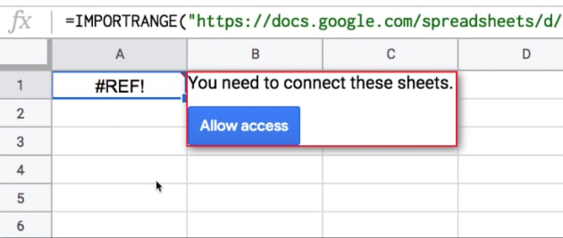
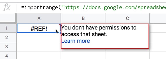
Initially, you’ll see a temporary #REF! error.

When prompted, click “Allow access” to grant access to the IMPORTRANGE function to import the data:

You only have to do this once.

Once access is granted, data from the source Sheet will appear in the destination Sheet.

Once two Sheets are linked with an IMPORTRANGE function, the data in the destination Sheet will update to reflect any changes made to the data in the source Sheet.

How To Use The IMPORTRANGE Function With Named Ranges

You can use the IMPORTRANGE function with named ranges.

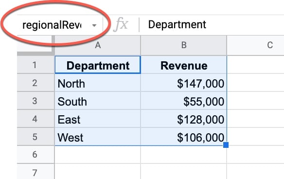
Suppose our source Sheet contains this named range: regionalRevenue

You can import the data in this named range by specifying the named range inside the IMPORTRANGE function.

Enter the full named range, between double quotes:

Google Sheets IMPORTRANGE Function Syntax

It takes two arguments:

spreadsheet_url

The URL of the source Google Sheet file, where you want to import data from.

range_string

A string specifying the range of data to import, enclosed in double-quotes.

It takes the format "[sheet_name!]range" e.g. "Sheet1!A1:D100"

If the Sheet name is omitted, the IMPORTRANGE function will import data from the first sheet of the source spreadsheet (i.e. the sheet furthest to the left).

IMPORTRANGE Function Notes

IMPORTRANGE is an external data function, which means it requires an internet connection to work.

Refresh Considerations

• Updates to the source Sheet will cause all destination Sheets to refresh.
• IMPORTRANGE waits for calculations in the source Sheet to complete before importing data.
• Sheets downloads the entire range specified in the IMPORTRANGE formula to your computer, so it will be affected by slow networks.
• There is a slight delay between making changes to a source Sheet and those changes showing in the destination Sheet.
• By default, the IMPORTRANGE function recalculates every 30 minutes (source).

Permissions

You need at least view-level access to other Sheets you want to retrieve data from.

If the source Sheet is from your own account, then you automatically have permission.

However, for external Sheets, you might not be able to import data without requesting access first.

If you don’t have permission, you’ll see the following error message: “You don’t have permissions to access that sheet.”

Access

Once access is granted, any editors in the destination Sheet can use IMPORTRANGE to import data from that source Sheet.

To remove access for an IMPORTRANGE function, remove the user who granted access from the source Sheet.

Array Output

The IMPORTRANGE Function in Google Sheets outputs an array, which means you can’t type over the top of the function output.

If you try to update the data from the IMPORTRANGE function, you’ll see a #REF! error “Array result was not expanded because it would overwrite data”:

Remember, the IMPORTRANGE function imports data from a different Sheet and displays a copy of it. So, changes need to happen in the underlying source Sheet.

Spreadsheet Key

The IMPORTRANGE function also works with the spreadsheet key instead of the full URL, although this is not commonly seen.

The spreadsheet key is the unique identifier that comes after the /d/ in the URL.

For example, this formula:

will give the same result as if we included the full URL:

You can copy the spreadsheet key from the URL bar of your source Sheet, although it’s easier to simply grab the whole URL and use that.

Best Practices With IMPORTRANGE In Google Sheets

To use IMPORTRANGE with data that expands in your source Sheet, use an open-ended reference (where you don’t specify an end row) to ensure new data is pulled through to the destination Sheet.

E.g. use range references without an end row reference, like this:

"Sheet1!A1:C"

instead of this:

"Sheet1!A1:C100"

Here are some tips to improve the performance of Sheets with IMPORTRANGE functions:

• Avoid chains of IMPORTRANGE formulas. Multiple layers of IMPORTRANGE will run slowly because changes automatically propagate through the chain, and cause delays at each step.
• Very large data imports may be slow, so consider performing analysis in the source Sheet and using IMPORTRANGE to import summarized results.
• For really huge data imports, you may need to look at Apps Script solutions, or even consider keeping data in BigQuery and using Connected Sheets to import into Google Sheets, instead of IMPORTRANGE.

IMPORTRANGE Function Template

Click here to open a view-only copy >>

Feel free to make a copy: File > Make a copy…

If you can’t access the template, it might be because of your organization’s Google Workspace settings.

In this case, right-click the link to open it in an Incognito window to view it.

The IMPORTRANGE function is also covered in the Day 18 lesson of my free Advanced Formulas 30 Day Challenge course.

It’s part of the Web family of functions in Google Sheets. You can read about it in the Google Documentation.