REPT Function in Google Sheets

The REPT function in Google Sheets is used to repeat an expression a set number of times.

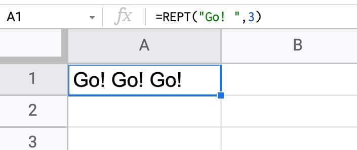
The REPT formula to repeat “Go! ” three times is:

Notice the additional space added after the exclamation point, so that there is a space between the repeated values in the output.

More REPT Function Examples

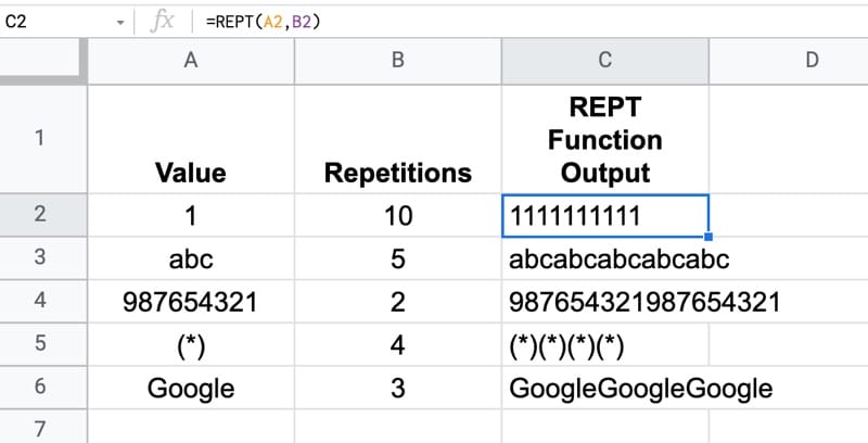
Column A contains the values you want to repeat.

Column B contains the number of repetitions.

The formula is then:

As you can see, for each row the value in A is repeated per the number in column B and joined into one long string.

REPT Function in Google Sheets: Syntax

The REPT function takes two arguments and both are required.

text_to_repeat

This is a text string or cell reference that you want to repeat.

number_of_repetitions

This is a positive integer indicating how many times you want to repeat the input text.

Notes on using the REPT function

• The return value (the output of the REPT function) is a string value in a single cell
• Setting the number of repetitions to 0 results in a cell containing a blank string (not a true blank cell though. ISBLANK will still give FALSE)
• Setting the number of repetitions to -1 results in a #VALUE! error
• If you want spaces between the repeated text strings, you must add that as the final character of the input string (as shown in the "Go! " example above). This results in a final trailing space, which can be removed with the TRIM function if required
• The number_of_repetitions can’t exceed the character limit of a cell: 32,000 characters. If it does, you’ll see a #VALUE! error
• Ranges can be repeated by wrapping the REPT function in an Array Formula

REPT function template

Click here to open a view-only copy >>

Feel free to make a copy: File > Make a copy…

If you can’t access the template, it might be because of your organization’s Google Workspace settings. If you click the link and open it in an Incognito window you’ll be able to see it.

You can also read about it in the Google documentation.

Using The REPT Function For Repeated Values In Separate Cells

What if you don’t want to create a long string of repeated values in a single cell, but instead want to output the repeated value across a range of cells, such that each value is in its own cell?

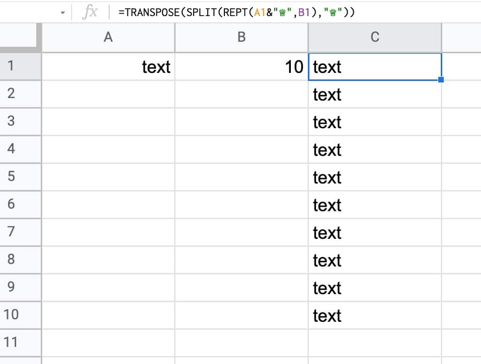
That’s possible with this formula, assuming the value is in cell A1 and the number of repetitions is in cell B1:

This particular formula outputs 10 values “text” in a column. (You can remove the transpose function if you want the output across a row.)

The Queen symbol “♕” is added to the end of the repeated value to act as a unique value used by the SPLIT function to divide the repeated string.

Note: you can also achieve this affect with the SEQUENCE function:

This particular variation uses the SEQUENCE function to output an array 1,2,3,…10. The TEXT function then “tricks” all of these to become empty strings. We then concatenate the repeated value from cell A1 onto this string. Finally, the Array Formula ensures that the output is an array.

Repeated Images with REPT Formula in Google Sheets

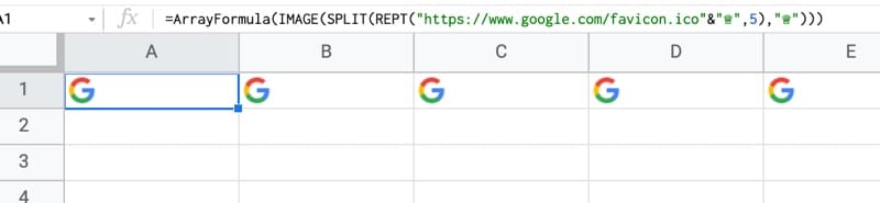
This REPT formula will repeat the specified image across a row. It uses the same Queen symbol “♕” trick as the previous formula.

The output looks like this:

Using REPT As Logical Formulas

The REPT function can be used instead of IF formulas in specific situations.

It’s quite a clever trick that works because TRUE is equivalent to the number 1, and FALSE to the number 0, in formulas.

So, by putting a logical test, which evaluates to TRUE or FALSE, equivalent 1 or 0, in the number of repetitions argument, we can either show 1 value or 0 values using REPT.

For example, this formula identifies values over $1,000:

And the output looks like this:

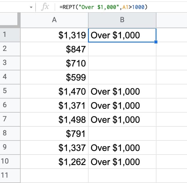
This formula works because the logical test checks if the value in cell A1 is greater than $1,000. If the result is TRUE, it’s interpreted as a value of 1, which then repeats the text in the REPT formula once. So the output is “Over $1,000”.

If the value is less than or equal to $1,000, then the test evaluates to FALSE, equivalent to 0 input for the REPT formula, so the output is a blank string in the cell.

This technique can be taken a step further to check multiple conditions are TRUE.

For example, the following formula checks whether the value is over $1,000 AND comes from Client A:

The two logical tests evaluate to TRUE or FALSE, which are interpreted as 1 or 0 by the formula.

When the value is greater than $1,000 and from Client A, it’s equivalent to:

In which case, the formula outputs the string “Over $1,000 and Client A”

Multiplication using “*” as shown above is for the AND case, where both conditions are true.

To do the OR case, you use addition “+”. If either value is TRUE and the other FALSE, it’s equivalent to 1 + 0 = 1. When both are true it’s equivalent to 1 + 1 = 2, so the REPT would repeat the value twice which we don’t want.

To fix this, wrap it with a MIN formula to set to 1 if the value is above 1.

In Cell Charts with REPT Function in Google Sheets

Bar chart with REPT Function

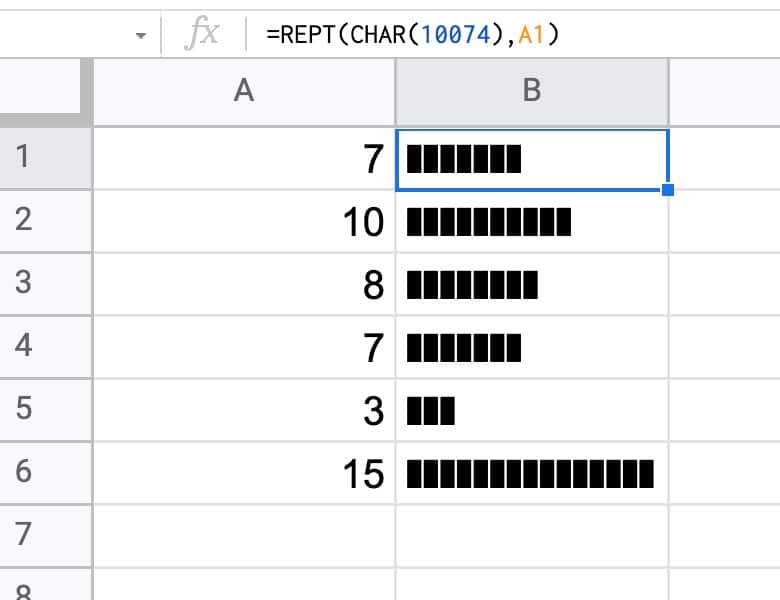
The formula to do this is:

The CHAR formula generates a special character based on the number.

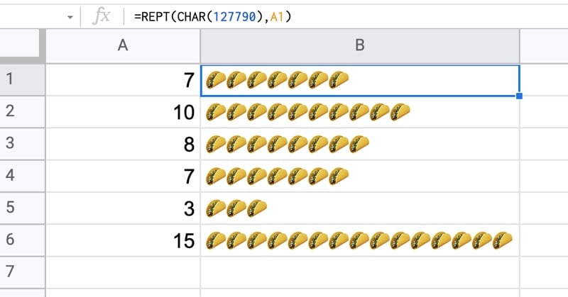
You can use any character as the repeated symbol, for example you could use tacos with CHAR(127790):

Vertical Bar Chart with REPT function

You can easily extend the technique above to display the bar chart in a single cell, with a vertical orientation, using this formula:

which looks like this (using dots as the repeated symbol):

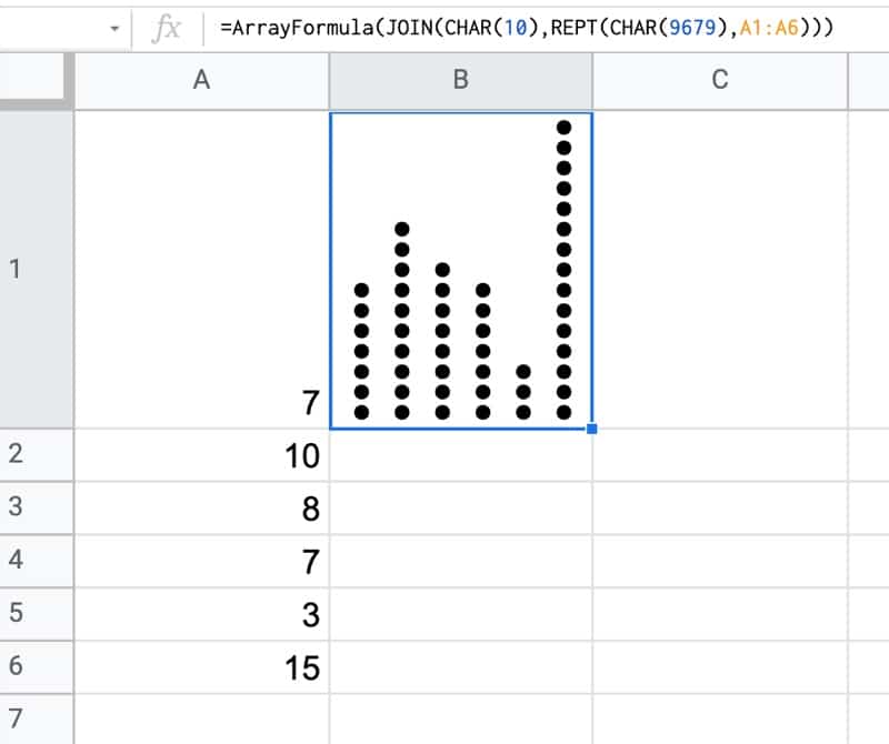
These charts are known as dot plots and you can find out more about how to create them here, including how to make them multi-colored: Dot Plots in Google Sheets

Dynamic Width Bar Charts Using REPT function

This is an interesting, although not particularly useful, formula which uses the CELL function to access the width of a cell and then sets the REPT to repeat the value to match the width of the cell:

The formula to do this is:

It uses the random number generator and the spreadsheet calculation setting to be “On change and every minute” to force the CELL function to re-calculate the width value each time there is a change.

The 1.25 factor at the end is simply to adjust the largest bar to fit the full width. It depends on the character you use to repeat and how wide it is. Feel free to experiment.

Padding Strings With The REPT Function

REPT can also be used to pad text strings.

With a value in A1, this formula adds a variable number of underscores to the end of the string:

If you want to have the text strings to have equal widths you’ll also need to use a font where the letters are equally spaced, like SOURCE CODE PRO.

This approach can also be achieved with numbers, although it’s much better to use custom number formatting, because that preserves the value as type number instead of converting to a string.