The TRANSPOSE function in Google Sheets interchanges the rows and columns of an array or range of cells in Google Sheets.
For example, suppose you are given data in a horizontal format like this:
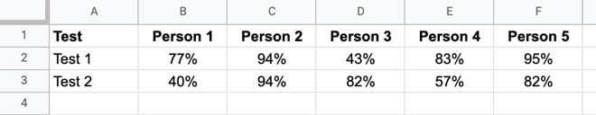
It’s awkward to read because it’s too wide to fit on a single screen. We’re also better at scanning down columns than across rows.
The TRANSPOSE function will flip the horizontal arrangement to a vertical arrangement:
=TRANSPOSE(A1:U3)like so:
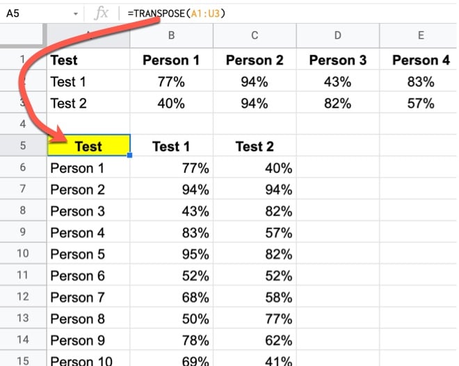
Much easier to use!
And it works better with other formulas like QUERY, SORT, FILTER, etc.
TRANSPOSE Function in Google Sheets Syntax
=TRANSPOSE(array_or_range)It takes a single argument: an array or range of cells.
Transposition works by swapping the row and column positions of each value. For example, a value in position row 3 column 10 will be put into position row 10 column 3 by the transposition operation.
As a result, ranges of size X rows and Y columns will become ranges of size Y rows and X columns.
In the screenshots at the top of this screen, the horizontal range with 3 rows and 21 columns became a vertical-oriented range with 21 rows and 3 columns.
It’s part of the Array family of functions in Google Sheets.
TRANSPOSE function template
Click here to open a view-only copy >>
Feel free to make a copy: File > Make a copy…
If you can’t access the template, it might be because of your organization’s Google Workspace settings. If you right-click the link and open it in an Incognito window you’ll be able to see it.
The TRANSPOSE function is also covered in the Day 25 lesson of my free Advanced Formulas 30 Day Challenge course.
You can also read about it in the Google Documentation.
TRANSPOSE Formula Examples
The TRANSPOSE function is useful in a wide variety of projects that make use of advanced formulas.
It pairs well with other text or array formulas, like the SPLIT function.
For example, maybe your data contains strings of comma-separated values in a cell that you want to present in column format. E.g. suppose you have an array of numbers in cell A1:
1,2,13,24,35,15,71
Then you can combine the TRANSPOSE function with the SPLIT function to achieve this:
=TRANSPOSE(SPLIT(A1,","))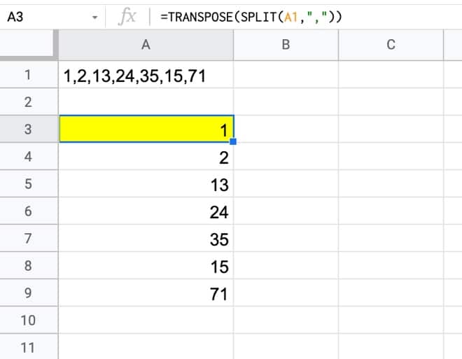
This post on how to alphabetize comma-separated strings uses this TRANSPOSE + SPLIT technique to break apart a string, before going on to sort the data and recombine.
Hi Ben,
Is there a way to multiple dynamic drop down boxes, to filter data being imported from a website, using either either importhtml or importxml. Eg d/e = 0% or > 0.05%.