In this post we’ll look at how to calculate a running total, using a standard method and an array formula method. We’ll cover the topic of matrix multiplication (take a deep breath, it’s going to be ok!) using the MMULT formula, one of the more exotic, and challenging formulas in Google Sheets.
If you like video tutorials, here’s the one on MMULT:
This is a lesson from my latest, Google Sheets course on Advanced Formulas 30 Day Challenge (it’s free!).
Running total dataset
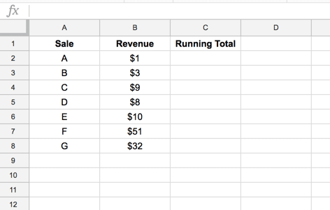
For the examples that follow, we’ll use this dataset:

We want to add a running total in column C.
Basic Running total
Let’s start off with the most basic method, using a standard (non-Array) formula which we can then copy down our column.
Taking the dataset above, we start our running total in cell C2, with this formula:
= B2It simply returns our first value, which is our only value at this stage.
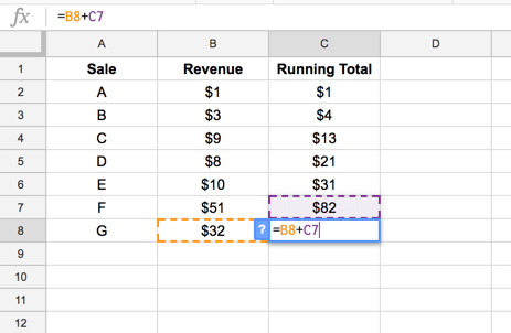
For our second value onwards, we can use the same standard formula, simply adding the new value to the running total from the line above:
= B3 + C2This formula can then be dragged down as far as required to give a running total:

If new items are added to the dataset, this formula will need to be dragged down further. Or you could pre-populate the column by dragging all the way to the bottom of your Sheet, and wrapping in an IF statement to hide on the blank rows, like so:
=IF(ISBLANK(B3), "", B3 + C2)The principal disadvantage of this formula is this need to fill out the entire column with a new formula for each row.
Wouldn’t it be nice if we could have a single formula at the top of the column to calculate the running total for us?
But first…
A quick aside on matrix multiplication
It’s been a while since I’ve done matrix multiplication, so I dug out one of my graduate mathematics books: Sets & Groups, A First Course in Algebra by J.A. Green.
Once I got over the initial shock of seeing “Ben Collins 1999” written on the inside cover (yes, I’m really that old!), I flipped to page 192 and reminisced about the good old days… no, I mean I refreshed my mind on the particulars of matrices, particularly their multiplication.
The only definition worth stating here, that pertains to the MMULT function, is this one:
The product AB of matrices A = (aij) and B = (bhk) is defined if and only if the number of columns of A equals the number of rows of B.
In other words if A has shape (m, n) then B must have shape (n, p), for this to work. The resulting matrix will have a shape (m, p).
Each entry in the new matrix is defined by the rule
(i, k) entry of AB = ith row of A * kth column of B
The MMULT formula does this matrix multiplication for us. It takes matrices A and B as arguments, =MMULT(A,B), and outputs the matrix product AB.
Phew, math aside, let’s get back to the more comfortable ground of our Google Sheet.
Array formula running total
Now you know how to do matrix multiplication, let’s use that in an array formula example with the MMULT function.
Let’s strategize before diving headlong into the formulas and note that:
1) A single row matrix, 1-by-X, multiplied by a single column matrix of compatible size, X-by-1, will result in a 1-by-1 matrix, i.e. a single value.
2) Taking this a step further, if the row matrix is {a,b,c} and the column matrix is {x;y;z}, then the product will be ax + by + cz, a single value, which is the sum of the elements multiplied together.
3) So, if we can get the values from our range in column B into a row format and multiply them by a column vector, we’ll be able to add them up!
4) The clever trick is to create a matrix 1 that only has the “correct” values in each row, so for row 1 it should only have the first value, for row 2 it should have the first two, for row 3 the first three etc. I.e. only the current or prior values in each row of our matrix.
5) Matrix 2 simply enables the multiplication to happen, so that the values can be added. So for this a vector of 1 would suffice.
Back to the problem at hand, using the dataset shared at the top of this post, let’s begin by constructing the two matrices for our MMULT function. I recommend restricting the range to B2:B10, to keep calculations manageable whilst we dissect the formula. Once we have a working formula, we can open up the range to B2:B.
Begin with this formula in cell E2:
=ArrayFormula(ROW(B2:B10))which simply gives us a column vector of the numbers 2 through 10, i.e. {2;3;4;5;6;7;8;9;10}
Add a TRANSPOSE function to the formula in cell F1:
=ArrayFormula(TRANSPOSE(ROW(B2:B10)))which simply transposes the column into a row vector of numbers, i.e. {2,3,4,5,6,7,8,9,10}
Now, let’s create a 9-by-9 matrix, by comparing these two vectors, and recording whether the value from the column vector is less than or equal to the value from the row vector, using:
=ArrayFormula(ROW(B2:B10) <= TRANSPOSE(ROW(B2:B10)))We should now have this output (color coding added):

which gives TRUE where the column vector value is less than or equal to the row vector value, and false otherwise.
Multiplying this by the original data range, B2:B10, turns the TRUE values into numbers and the FALSE values into zeros:
=ArrayFormula((ROW(B2:B10) <= TRANSPOSE(ROW(B2:B10)))*B2:B10)to which we apply a TRANSPOSE function again, to flip the data into the correct orientation
=ArrayFormula(TRANSPOSE((ROW(B2:B10) <= TRANSPOSE(ROW(B2:B10)))*B2:B10))so that the values from our data range in B2:B10 are now sitting in a 9-by-9, correctly starting from their corresponding row (so value in B2 starts in row 2, value in B3 starts in row 3 etc.), as shown in this image:

So that’s matrix 1 ready for the MMULT formula.
Let’s construct matrix 2. Thankfully it’s a little simpler:
=ArrayFormula(SIGN(B2:B10))which creates a 9-by-1 matrix, or column vector, where any positive numbers in the range B2:B10 return 1, and blank cells return 0, so the end result is our column vector {1;1;1;1;1;1;1;0;0}
Plug these both into the MMULT function and watch the magic happen:
=ArrayFormula(MMULT(TRANSPOSE((ROW(B2:B10)

 <= TRANSPOSE(ROW(B2:B10)))*B2:B10),SIGN(B2:B10)))
Recall, from matrix multiplication, our 9-by-9 matrix multiplied by our 9-by-1 matrix results in a new 9-by-1 matrix.
Each element in the first row of matrix 1 is multiplied by the column values in matrix 2, and added together, which if I try to illustrate, looks like this:
The first row of matrix 1 is {1,0,0,0,0,0,0,0,0}
The first column of matrix 2 is {1;1;1;1;1;1;1;0;0}
Therefore the first value in the new matrix is:
1*1 + 0*1 + 0*1 + 0*1 + 0*1 + 0*1 + 0*1 + 0*0 + 0*0

= 1 + 0 + 0 + 0 + 0 + 0 + 0 + 0 + 0

= 1
(You may have noticed that this is a 1-by-9 matrix multiplied with a 9-by-1 matrix, resulting in a 1-by-1 matrix, or simply, a single value.)
Correspondingly, row 2 calculation:
1*1 + 3*1 + 0*1 + 0*1 + 0*1 + 0*1 + 0*1 + 0*0 + 0*0

= 1 + 3 + 0 + 0 + 0 + 0 + 0 + 0 + 0

= 4
Row 3:
1*1 + 3*1 + 9*1 + 0*1 + 0*1 + 0*1 + 0*1 + 0*0 + 0*0

= 1 + 3 + 9 + 0 + 0 + 0 + 0 + 0 + 0

= 13
Etcetera, to our desired output of:
{1;4;13;21;31;82;114;114;114}
So this formula gives the running total.
The final step is to only show it on non-blank rows, which we achieve with standard IF logic.
Here I’ve used this IFERROR function construction
IFERROR(1/0)to ensure the cells are blank whenever range B2:B10 is blank. 1/0 always results in a #DIV/0! error so the iferror wrapper then leaves the cell blank.
So our formula is now:
=ArrayFormula( IF(B2:B10,MMULT(TRANSPOSE((ROW(B2:B10)<=TRANSPOSE(ROW(B2:B10)))*B2:B10),SIGN(B2:B10)), IFERROR(1/0)))which can be generalized to the whole of column B, by removing the 10 row reference from B2:B10.
Our formula in its final state is:
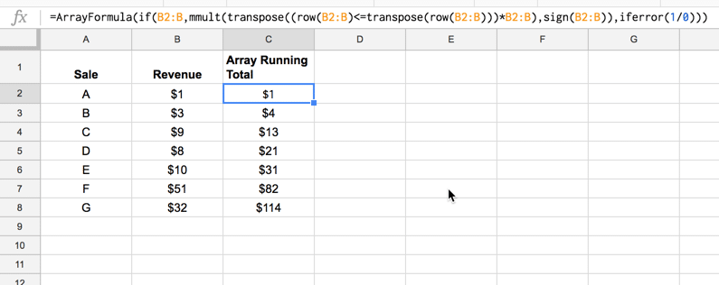
=ArrayFormula(IF(B2:B,MMULT(TRANSPOSE((ROW(B2:B)<=TRANSPOSE(ROW(B2:B)))*B2:B),SIGN(B2:B)), IFERROR(1/0)))as shown in the following screenshot:

If new rows of data are added in columns A and B, the running total column will update automatically.
Can I see an example worksheet?
Bonus: conditional array formula running total
This is really just a proof-of-concept idea.
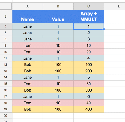
It’s possible to create a single array formula that creates separate running totals for each unique item in Column A, up to 9 unique items, as shown in this image:

The formula for this is a complete beast (and I’m not saying this is the only, or best, way of achieving this):
=ArrayFormula(query(query(if({transpose(unique(indirect("A6:A"&counta($A$6:$A)+1)))}=$A$6:$A,mmult(transpose((row($B$6:$B)<=transpose(row($B$6:$B)))*$B$6:$B),if({transpose(unique(indirect("A6:A"&counta($A$6:$A)+1)))}=$A$6:$A,1,0)),0),"select "&left(concatenate(transpose("Col"&row(indirect("1:"&countunique($A$6:$A)))&"+")),countunique($A$6:$A)*5-1)&" label "&left(concatenate(transpose("Col"&row(indirect("1:"&countunique($A$6:$A)))&"+")),countunique($A$6:$A)*5-1)&" ''",0),"select * limit "&counta(A6:A)))Needless to say, I’m not going to break that out line by line, at least not today.
It makes use of the INDIRECT function to convert strings into valid range references and the UNIQUE function to remove duplicate values.
If you’re interested, the best way to approach it is to peel back the layers, using the onion method in Google Sheets, until you reach the inner most formula, and then build it back up.
Good luck!
Wow. I got lost here pretty quickly, after ‘Array formula running total’. Why are you multiplying numbers (and why ROW numbers, at that?) when you want to be adding numbers? Could you explain how you decided that this problem needed a matrix multiplication solution in the first place? Thanks.
Hey Gary,
I’ve added some more notes to the start of that section, which will hopefully give some insight. The key is knowing the inner workings of matrix multiplication, specifically that if the row matrix is
{a,b,c}and the column matrix is{x;y;z}, then the product will beax + by + cz, a single value, which is the sum of the elements multiplied together.So basically we create rows containing the values from B up to the current row, and multiply each row against a column of 1’s which then adds up those values for each row (to give the cumulative total).
Hope that helps.
Cheers,
Ben
Great, that helps me!
I hadn’t done matrix multiplication for decades, and I managed to skim read over the bit were you said after the multiplication the numbers are added together
Great! Thanks for your original question too. I had made a leap there without explaining why, so you’ve helped improve the post 🙂
I really like how that works, but what do you need to change to include negative values?
Great Ben, this amazing, Thank you.
Can you help me understand why the formula doesn’t work with negative values? I mean, when adding cell B2=-300 to cell B3=600 the formula outputs 900 instead of 300. Also it is blank when a zero is in the B column instead of keeping the value from the previous row. I know you kinda covered this in your post, but I still don’t get it. Please help.
Hey Matt,
You’re right, it breaks down for negative numbers. The issue is that the two matrices we create will both contain the negative value (the SIGN function returns a negative number), which multiplied together give a positive number.
However, you can change the sign function to this construction to get around this. So change:
sign(range)to:
if({range}<>0,1,0)I’ve added the full updated MMULT formula to the linked template from the article.
Re the blank: It’s blank because we have an IF wrapper function which sets the output to blank if the value is blank (so it stops showing the total when we reach the last row). It was envisaged working with a continuous column of data. You could probably tweak it to fill in blank gaps if you wanted…
Hope that helps!
Cheers,
Ben
another trick when dealing with +/- 1, is to change:
SIGN(range)
to:
SIGN(range)^2
Is this method advantageous in some way to using a SUMIF formula instead?
Column-wise:
=ARRAYFORMULA(IF(A2:2,SUMIF(COLUMN(A2:2),”<="&COLUMN(A2:2),A2:2),IFERROR(1/0)))
Row-wise:
=ARRAYFORMULA(IF(B2:B,SUMIF(ROW(B2:B),"<="&ROW(B2:B),B2:B),IFERROR(1/0)))
This certainly seems to be less taxing on the recalculation.
Can’t seem to get this to work.
That’s a very elegant solution, and a lot simpler than using MMULT.
This works. Is there some documentation to explain how column() and row() seem to behave differently in arrayformula (that is, they seem to be returning a multicell range)?
They still behave the same, returning an integer for the row (or column) reference. Inside an array formula though, they loop over all the rows (or columns) specified in the range, so you can access each row (or column) in turn in your calculations.
yeah I spotted that it breaks for negative nums too, fixed it by
replaceing sign(range)
with
sign(range)*sign(range)
but I think the if statement is clearer. cheers
Hey thanks for the formula.
Has anyone noticed it breaking down when you more than 10 unique value in the first column.
Hey Stewart,
You’re referring to that final conditional formula right? Great spot! It does appear to break on the 10th unique item so I’ve added that caveat to the post above.
There are simpler (and probably better) ways to solve the problem tbh, like a pivot table for example…
Thanks for letting me know.
Ben
I’ve got a large dataset that has more than 9 unique conditions. I would prefer to utilize an arrayformula instead of a pivot table. I’ve been trying to wrap my head around why that formula would cap out at 9. Is it possible to have more (if not an unrestricted amount) unique conditions on this running total?
hi all,
apologies for what must be a silly question, but please may i enquire why a simple ‘sum’ formula (e.g. =sum($A$1:A1) ) wont work as well?
Thanks
Hey Abdul,
This method allows you to place a single formula at the top of the cumulative total column that will calculate the running total for any non-blank rows.
Sometimes simple is better though, in which case you could use the formula you suggested and copy down.
Thanks!
Ben
I’ve got a large dataset that has more than 9 unique conditions. I would prefer to utilize an arrayformula instead of a pivot table. I’ve been trying to wrap my head around why that formula would cap out at 9. Is it possible to have more (if not an unrestricted amount) unique conditions on this running total?
I have my spreadsheet filled in. one column with names (A). then the next with amounts (B). I managed to total the column (B). it worked correctly. Then now I need to continue with more data, that total line, took a space, and when I add in new info, it basically is starting over. I intended to be able to add more daily, and keep it at a running total. How do I fix it?
Hi Ben, how would you adapt your proposed running total array solution to use in a moving average solution, where you can specify a moving average of n periods?
Hi Ben,
Grateful for your post 🙂 – Now that you’ve blazed a trail for us, I just changed sign(b2:b) for abs(sign(b2:b)) to allow for negatives.
I also like Daniel’s solution – thanks Daniel!
Hi Ben,
Really interesting formula.
I have however a question. Could this formula be modified to have an inverted running sum (so it starts counting from the bottom)?
I tried putting a SORT(descending) function in the output, but that drags all cell to the top and removes the blank cells in between, thus the sum is not in line with the date.
Thanks in advance!
Nick
very clever. Nice hack.
Hi Ben,
This is very well explained! I tried to play with these concepts to implement a running high water mark combining the max function with your tips. To stay with your sample data, if the high water mark column were in column D, its content should be:
{1;3;9;9;10;51;51}, i.e. the highest revenue so far when going down the column.
This is part of a goal to emulate subtotal() with array functions to avoid having to duplicate subtotal() calls across rows (or columns). I’ve been able to figure out how to do it for sum, average, count, counta, but I’m stuck on max/min. Is this something you cover in your courses ?
Thanks in advance,
– jr
Sir,
Good day,
i am now making a statement of account using google sheet, i am using Query to show the detail of Account receivable from certain customer, I find it hard to show the payment made by the customer, using query on my format,
i want it to show like this.
date Invoice No. Particulars Invoice amount Payment Balance
3-6-19 123456 sales 10,000 10,000
3-8-19 123456 Payment 10000 0.00
please help
Thanks for this Ben, really useful.
One thing I noticed though is if the source data contains zeros, the running total is blank for those rows, rather than maintaining the running count.
The way I solved this was to simply duplicate the MMULT function, and restrict it from running on for the entire length of the column by checking if the source row ISBLANK()
I’m sure someone will improve on this, but it’s solved my problem for now…
Forgot to include the formula! 🙂
=ArrayFormula(if(isblank(Q3:Q),,IF(Q3:Q,MMULT(TRANSPOSE((ROW(Q3:Q)<=TRANSPOSE(ROW(Q3:Q)))*Q3:Q),SIGN(Q3:Q)), MMULT(TRANSPOSE((ROW(Q3:Q)<=TRANSPOSE(ROW(Q3:Q)))*Q3:Q),SIGN(Q3:Q)))))
Thank you for this
In my case the running total don’t become blank rows. Could you please share a sample sheet to illustrate the problem? Thanks!
Came looking for a magical way to do running totals. The MMULT way is indeed magical, but it really serves to illustrate the dangers of complex spreadsheets, given that the initial formula only worked for a very limited dataset and then broke down in fun and interesting ways. I would hope my doctor/aeronautical engineer/finance department did as I did and used the KISS method that you start with. 🙂
The formula doesn’t seem to work for me. I get the error that the “resulting array is too large.” I have only 47 rows so far.
I’ve tried down to 200 rows without the “array too large” error.
May I suggest a few alterations to the original formula:
‘
=ArrayFormula(IF(B2:B=””,,MMULT(TRANSPOSE((ROW(B2:B)<=TRANSPOSE(ROW(B2:B)))*B2:B),ABS(SIGN(B2:B)))))
'
This avoids the "blank with 0" problem as well as the negative number problem, without adding any queries or extra tests.
I offer alternative for last huge formula:
=ArrayFormula(MMULT((ROW(A6:A19)>=TRANSPOSE(ROW(A6:A19))) * EXACT(A6:A19,TRANSPOSE(A6:A19))^1, (B6:B19)^1))
awesome, this works and it is so simple
Thanks, Ben, this is good stuff.
I fixed two more things to make it universal in my sheet:
1. used ISBLANK, to make it work for 0 values, as suggested by DJE
2. used SIGN(range)^2 to care for negative values, as suggested by Dan
Final formula, which I hope us useful to someone:
=ARRAYFORMULA(IF(ISBLANK(D3:D);IFERROR(1/0);MMULT(TRANSPOSE((ROW(D3:D)<=TRANSPOSE(ROW(D3:D)))*D3:D);SIGN(D3:D)^2)))
Replace D3:D with your (open ended) col.
If for some reason you want to do running total ROW-wise this is the formula that works for me when you have a POSITIVE range of values starting from D1 all the way up to columns running over row 1
“`
=ArrayFormula(if(D1:1,transpose(MMULT(transpose((transpose(COLUMN(D1:1))<=COLUMN(D1:1))*transpose(D1:1)),SIGN(transpose(D1:1)))),iferror(1/0)))
“`
Being into finance function, this was the biggest challenge for me always. To display running totals/balances. Thankfully we have you, Ben. And to be honest, I just copied the formula and solved my thing, didn’t get to understand every layer of it 🙂
Hi, i really need your professional advise
i using this formula
=ARRAYFORMULA(IF(LEN(M3:M), M3:M&” – “&
MMULT((M3:M = TRANSPOSE(M3:M)) * (ROW(M3:M) >= TRANSPOSE(ROW(M3:M))),
SIGN(ROW(M3:M)))+0, IFERROR(1/0)))
but came out error message:
Error
The resulting array was too large.
Please help….
If your table has continues dates you can replace all “M” for “INDEX($M$3:$M,COUNTA($M$3:$M)-1)”.
The formula is going to be:
=ARRAYFORMULA(IF(LEN(M3:INDEX($M$3:$M,COUNTA($M$3:$M)-1)), M3:INDEX($M$3:$M,COUNTA($M$3:$M)-1)&” – “&
MMULT((M3:INDEX($M$3:$M,COUNTA($M$3:$M)-1) = TRANSPOSE(M3:INDEX($M$3:$M,COUNTA($M$3:$M)-1))) * (ROW(M3:INDEX($M$3:$M,COUNTA($M$3:$M)-1)) >= TRANSPOSE(ROW(M3:INDEX($M$3:$M,COUNTA($M$3:$M)-1)))),
SIGN(ROW(M3:INDEX($M$3:$M,COUNTA($M$3:$M)-1))))+0, IFERROR(1/0)))
However it doesn’t work if you have empty spaces in the range.
I want to multiply the values in the row instead of sum. Something like:
Row 3
= 1 * 3 * 9 * 1 * 1 * 1 * 1 * 1 * 1
= 27
To convert 0 to 1 I used IF statement in the formula, like this:
=ARRAYFORMULA(IF(TRANSPOSE((ROW($S$4:INDEX($S$4:$S,COUNTA($S$4:$S)-1))<=TRANSPOSE(ROW($S$4:INDEX($S$4:$S,COUNTA($S$4:$S)-1))))*$S$4:INDEX($S$4:$S,COUNTA($S$4:$S)-1))=0,1,TRANSPOSE((ROW($S$4:INDEX($S$4:$S,COUNTA($S$4:$S)-1))<=TRANSPOSE(ROW($S$4:INDEX($S$4:$S,COUNTA($S$4:$S)-1))))*$S$4:INDEX($S$4:$S,COUNTA($S$4:$S)-1))))
Is it possible to multiply instead of sum?
I did it with filter:
FILTER(IF(S4:S20=””,IFERROR(1/0),MMULT(TRANSPOSE((ROW(S4:S20)<=TRANSPOSE(ROW(S4:S20)))*S4:S20),SIGN(S4:S)^2)),S4:S20″”)
It works fine with limited range, however it doesn’t work with unlimited range:
FILTER(IF(S4:S=””,IFERROR(1/0),MMULT(TRANSPOSE((ROW(S4:S)<=TRANSPOSE(ROW(S4:S)))*S4:S),SIGN(S4:S)^2)),S4:S””)
In my Google sheets it gives me a error “the array was too large”.
Sure, if I wanted to play mental gymnastics all day, these types of solutions would be great. But I don’t want to create something that is unsupportable. As spreadsheets/formulas become more complex, I start liking them less and less.
I need to display/return in the line in front of the action code EKTR4 the corresponding values of Nº Trades for each date/reference in the range B1:AP1.
But it is required to return/display zero(0) when there is no trade/corresponding date of action EKTR4.
Please how do I do this?
The range/array was obtained from the following query: INDEX(SE(QUERY(IMPORTHTML(CONCAT(“https://www.ibovx.com.br/historico-papeis-bovespa.aspx?papel=”;A5);”table) “;0);”Select Col1 where Col1 IS NOT NULL LIMIT 41 LABEL Col1””)=B1:AP1;QUERY(IMPORTHTML(CONCAT(“https://www.ibovx.com.br/historico-papeis-bovespa .aspx?papel=”;A5);”table”;0);”Select Col9 where Col9 IS NOT NULL LIMIT 41 LABEL Col9””);0))
Here’s the link to the spreadsheet to make it easier:
https://docs.google.com/spreadsheets/d/1tC3sdATEaCr1VW2MLJyy1sPYwkvCoF63cOp2YM0ZzHQ/edit?usp=sharing
I’m from Brazil, forgive me if the translation is wrong.
Thanks.
Hello! I found out how. It was simpler than I imagined: Query( data range you quote; “Select MAX(Col1), MAX(Col2),…… MAX(LAST COLUMN)”).
Sometimes we think the problem is very difficult, but it is simpler.
Thanks!
In a similar way, I’m trying to calculate a running total for hours used in a month, when you can banked unused hours from your monthly allocation for up to 3 months. Banked hours can be used in a first in first use basis.
Example
Month Allocation Used Delta Carry over from previous month.
Jan. 15. 11 4 0
Feb. 15 14 1 4
Mar. 15 12 3 4+1
Apr. 15 13 2 4+1+3
May 15 19 2 (Jan hrs dropped, use 2 hrs carried over)
June 15 18 1
Any ideas tips on how to achieve this using formulas would be greatly appreciated.
Thanks
Yann
Hey Ben,
Thanks for a great solution! I have been looking for it for many weeks. Meanwhile, it is limited by 9 unique records (don’t understand why). Is there any workaround to implement such solution for unlimited records (it could be up to 500 in my case)?
Many thanks.
You might have some joy with the SCAN function: https://www.benlcollins.com/spreadsheets/scan-function/
I haven’t done it for different unique records, but it works a treat for running totals, so I think it would be worth an explore.
Ben