The UNIQUE function in Google Sheets is a hugely useful function that takes a range of data and returns the unique rows and discards the duplicate rows.
Here’s a super simple example to show how it works:
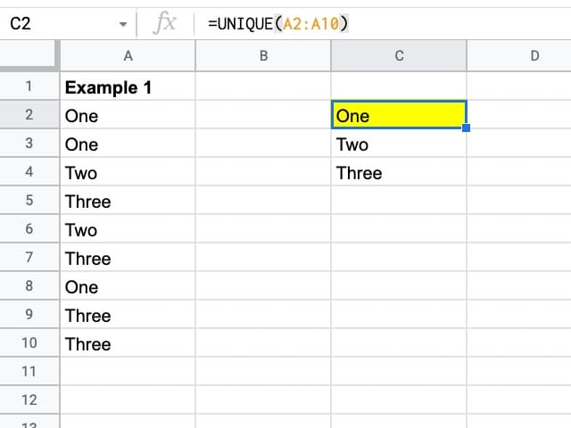
Here, the data from column A is passed into the UNIQUE formula and the unique values are returned.
UNIQUE Formula Example
Let’s see another example, using data showing the world’s top chess players:
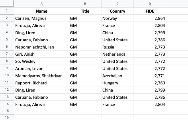
Unfortunately, there are duplicate rows in the dataset. Can you spot them?
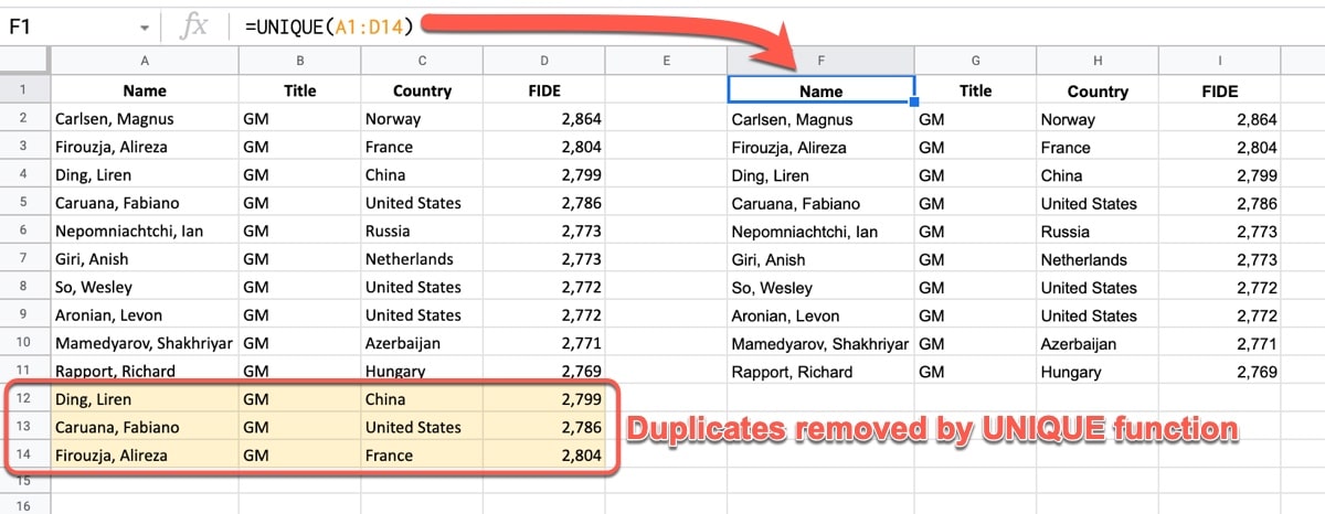
Thankfully the UNIQUE function can easily remove the duplicate rows:
=UNIQUE(A1:D14)Moreover, it returns the remaining rows in the same order as in the original dataset.
UNIQUE Function Syntax
=UNIQUE(range)It takes a range or list of data as a single argument.
UNIQUE is part of the Filter family of functions in Google Sheets.
Function Notes
The order of the original rows is preserved with the UNIQUE function. In other words, it doesn’t perform any sorting operations on your data.
However, we need to be careful with mixed data columns. What looks different to us might be the same for the UNIQUE formula.
Consider this example of a column containing the value 1 formatted in 3 different ways:
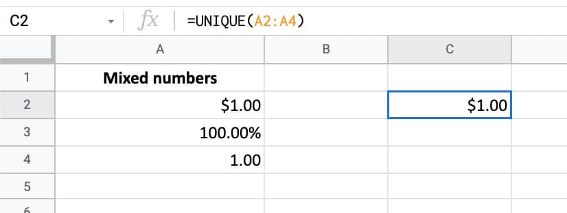
The values are all 1, but they’re formatted differently.
Therefore UNIQUE throws away the two duplicate values and takes the formatting from the first value.
UNIQUE Function Template
Click here to open a view-only copy >>
Feel free to make a copy: File > Make a copy…
If you can’t access the template, it might be because of your organization’s Google Workspace settings. If you right-click the link and open it in an Incognito window you’ll be able to see it.
You can also read about it in the Google Documentation.
Advanced UNIQUE Formula Example
The major benefit of the UNIQUE function over other methods of removing duplicates – e.g. the menu – is that it can be nested inside other formulas.
In other words, it can be part of a formula algorithm.
Consider this example dataset:
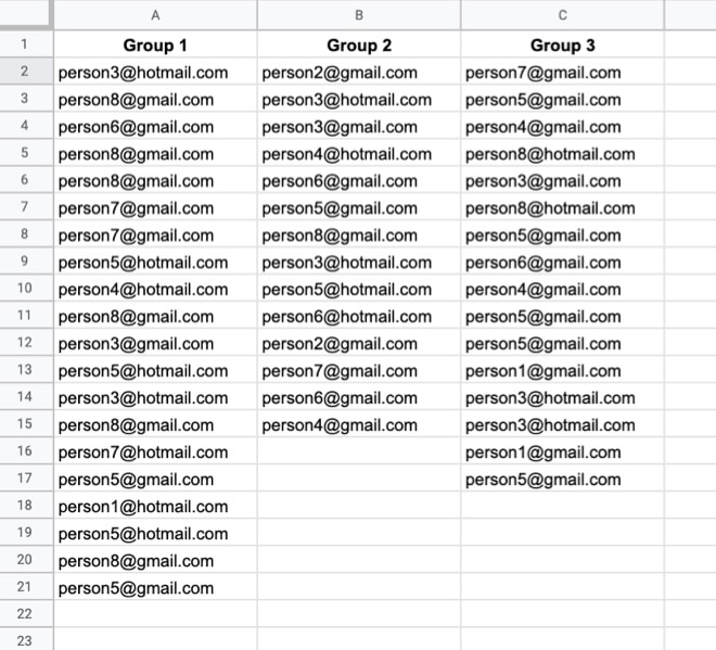
Here we collected email addresses from attendees at three separate events.
There is some overlap between the emails, so we want to remove the duplicate email addresses when we combine the lists.
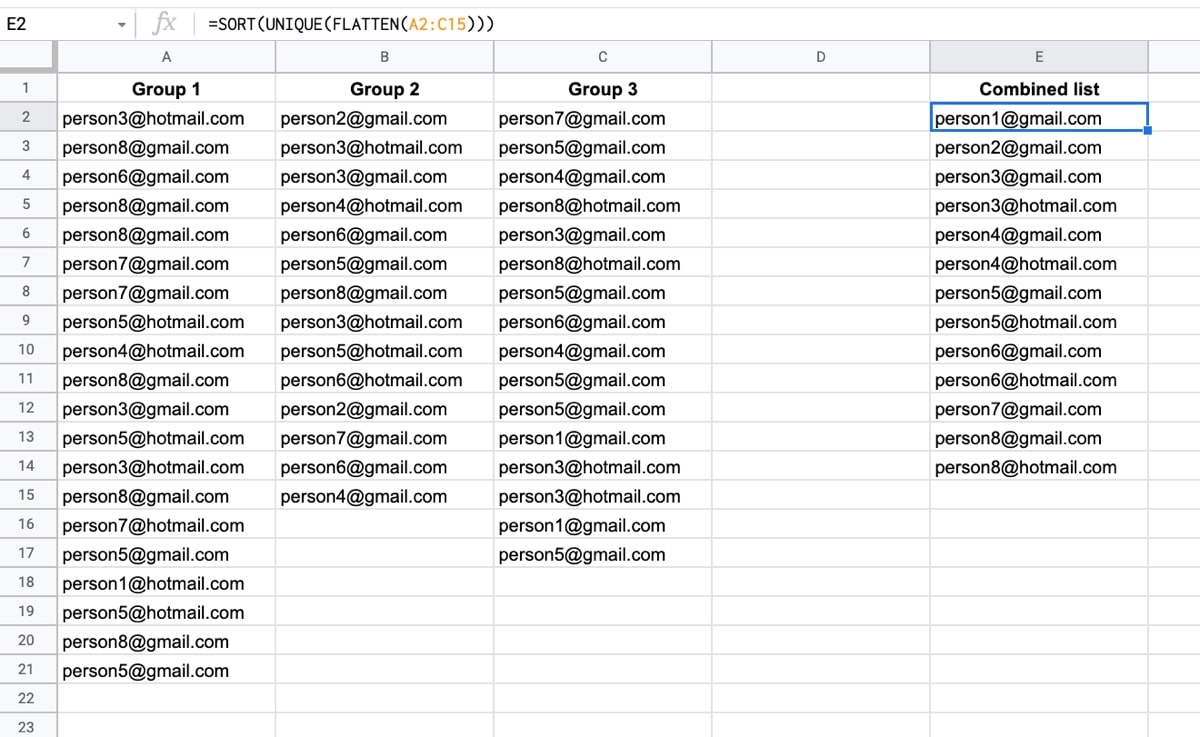
This formula creates a unique list of email addresses:
=SORT(UNIQUE(FLATTEN(A2:C15)))How does this formula work?
It uses the FLATTEN function to combine the columns.
Then UNIQUE removes any duplicates before the SORT function sorts the result alphabetically.
Here’s another advanced example involving the UNIQUE function:
I have a table of data when col1 is a unique key and col2-10 is updates on the key,
key1,date,test,result,action,duration
key1,date2,test2,result2,action,duration
key1,date3,test3,result3,action,duration
key2,date1,test1,result1,action,duration
key2,date2,test2,result2,action,duration
key3,date1,test1,result1,action,duration
key3,date2,test2,result2,action,duration
key4,date1,test1,result1,action,duration
key4,date2,test2,result2,action,duration
I want to get a report of unique keys and the entire first row of the data.
Usually I just put =unique(col1) in col1 of my report and in col2 put vlookup(col1,data!a:j,{2,3,4,5,6,7,8,9,10},0) and that gets me the 1st instance of col1 and the following data. Is there a shorter way to write that? perhaps with a query?