This post shares my solution to a problem that I faced myself recently.
I needed the unique list of items from a column containing grouped words, separated by commas.
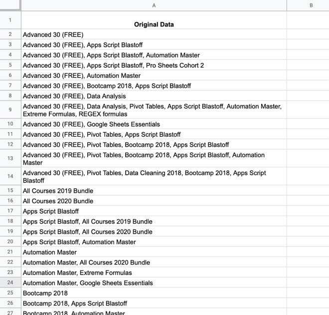
The data was in this format:

As you can see, it’s a list of my online courses, but many of the rows contain more than one item, separated by commas.
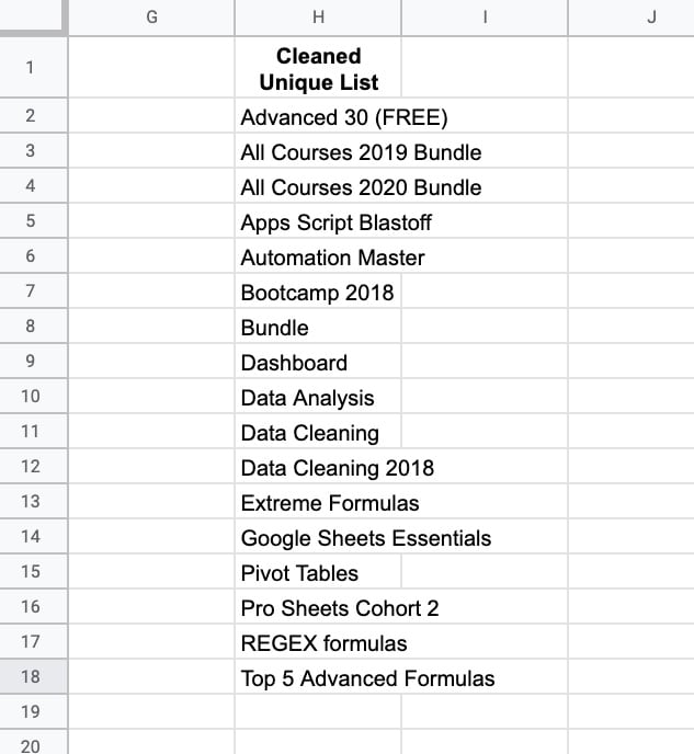
Ultimately, I want to transform the data into this format:
Formula To Create A Unique List Of Items
Enter this formula in a blank column to create the unique list of items:
=ArrayFormula( QUERY( UNIQUE( TRIM( FLATTEN( SPLIT(A2:A100,",")))),"where Col1 is not null order by Col1"))How Does This Work?
Let’s use the onion method to peel the formula apart.
Step 1:
Start with the innermost SPLIT function to separate items in the rows with multiple items:
=SPLIT(A2:A100,",")We’re telling the SPLIT function to separate items based on the commas.
Step 2:
Turn this into an array formula to capture all of the original rows:
=ArrayFormula(SPLIT(A2:A100,","))Step 3:
Next, add the FLATTEN function to combine all the columns into a single column:
=ArrayFormula(FLATTEN(SPLIT(A2:A100,",")))Step 4:
Then add the TRIM function to remove any superfluous whitespace around the text values, to ensure we can remove duplicates:
=ArrayFormula(TRIM(FLATTEN(SPLIT(A2:A100,","))))Step 5:
Almost there…!
Wrap the formula with the UNIQUE function, which will remove the duplicate values:
=ArrayFormula(UNIQUE(TRIM(FLATTEN(SPLIT(A2:A100,",")))))Step 6:
Finally, we’re ready to extract the unique list of items 😉
Add the QUERY function as the final layer, to sort the data and remove the blank row:
=ArrayFormula( QUERY( UNIQUE( TRIM( FLATTEN( SPLIT(A2:A100,",")))),"where Col1 is not null order by Col1"))One interesting thing you’ll notice about this QUERY function is that it doesn’t contain a SELECT keyword. That’s because I’m selecting all of the columns, so, for brevity, I omitted the SELECT statement.
The QUERY statement is functionally equivalent to:
"select * where Col1 is not null order by Col1"You’ll also notice that the QUERY statement uses the Col1 notation, rather than referring to columns with A, B, C notation. That’s because the data input for the QUERY function is generated by another function, nested inside the QUERY.

We do a huge survey at the end of the year for Title 2 (professional development) funding. We ask teachers across several different campuses what topics they want to learn about in the coming year. This causes similar lists with commas that I have to analyze.
1) OMG I’m so glad you shared about the Flatten Formula! I’ve been looking for that (and not knowing how to search for it) for years! Thank you Thank you Thank you! I can google for just about anything, but I can’t figure out how to google for “I need a formula that would accomplish such and such.”
2) The formula you share here is useful to get all the unique responses from a survey. I’m hoping you can share in the future how to then analyze “how many teachers from CampusA responded with Option1?” Curious to see how my method compares to yours.
A2:A65 includes all the possible choices.
B column is for totals
C1:Z1 are the campus names
Here’s the formula I use to count the responses for each campus:
=countifs(CurrentData!$C$2:$C$2188,C$1,CurrentData!$F$2:$F$2188,concatenate(“*”,$A26,”*”))
The data is on sheet CurrentData, the campus is in column C and the question is located in column F.
3) Another analysis that I’m wondering about: How to convert your data into multiple columns. So you see each person on the left and each column represents one of the responses: PersonA has “yes” in columns B, C and E because they chose those responses from the survey.
3b) Then you can analyze How many people chose both B and E. (I’m not sure how to do either of these efficiently)
I could probably accomplish questions 2 & 3 with pivot tables; unfortunately, I’ve never been able to get my head around how they work.
Thank you so much for all you share!
Hi Amber,
I would potentially be able to help you out if you would be able to share a sample copy of your spreadsheet?
Make sure it doesn’t contain any sensitive information or if any, replace them with false ones.
Cheers
I have 5 columns of data, a:e( date, location, event1, event2, event3), and I want to return unique values for column B (location) but the rest of the columns still appear that would be with that row.