The TRIM function in Google Sheets removes unwanted spaces around text.
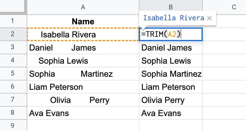
TRIM removes the leading, trailing, and repeated spaces in the text values in column A.
The formula is:
=TRIM(A2)🔗 Get this example and others in the template at the bottom of this article.
TRIM Function Syntax
=TRIM(text)It takes a single argument which is a string or reference to a cell containing a string.
TRIM Function Notes
TRIM removes all spaces in a string to leave only single spaces between words.
The TRIM function combines well with other functions to ensure consistent data at each step.
It’s also really useful for data cleaning to ensure that values are identical.
TRIM Function Explained
Let’s look at the first example in more detail.
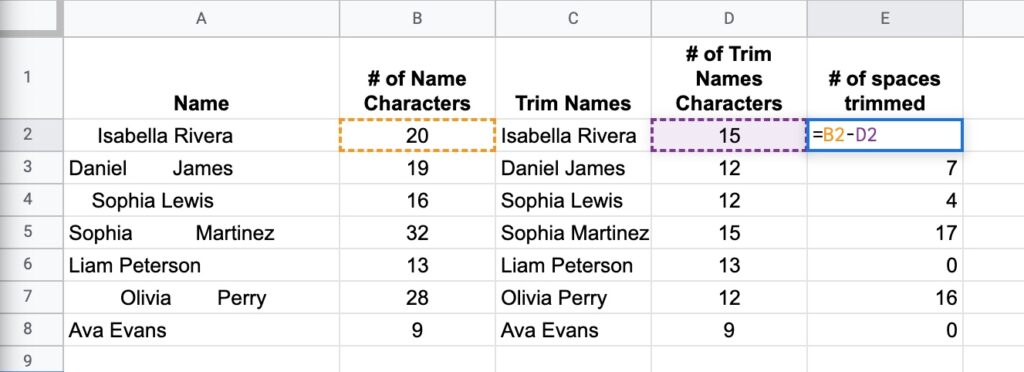
We’ll use the LEN function to count how many characters are in a cell, before and after applying the TRIM function. Then we’ll subtract these two values to see how many spaces TRIM removed.
With the names in column A, add these formulas in adjacent columns:
In B2, to count the length of original data:
=LEN(A2)
Then in C2, to trim the data:
=TRIM(A2)
And in D2, to count the length of the trimmed data:
=LEN(C2)
Finally, in E2, to count how many spaces were removed:
=B2-D2
Here’s what this looks like in the Sheet:
TRIM Function Example
Suppose you have the following dataset:
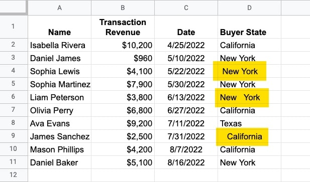
Look at the yellow highlighted values in column D. Something is slightly wrong with them.
They have spaces before the names or too much whitespace between the “New” and “York”.
This is a problem because they will be treated as different values by the computer, even though we know they’re the same.
Consequently, you’ll get bad results if you try to summarize this data because the values are inconsistent.
TRIM will fix these whitespace issues so that all the values are consistent.
In this example, this simple TRIM formula fixes the whitespace issues in column D:
=TRIM(D2)Furthermore, you can use the TRIM function as an array formula to fill down the range automatically with this single formula:
=ArrayFormula(TRIM(D2:D11))Array formulas like this work particularly well with Google Form data, where you might leave the range reference open (i.e. D2:D) so it expands with your data:
=ArrayFormula(TRIM(D2:D))Advanced TRIM Formula Uses in Google Sheets
The TRIM function is really useful for data cleaning work. It combines well with other functions to ensure consistent data at each stage of a project.
Consider this example, which is creating a unique list from the values in column A:
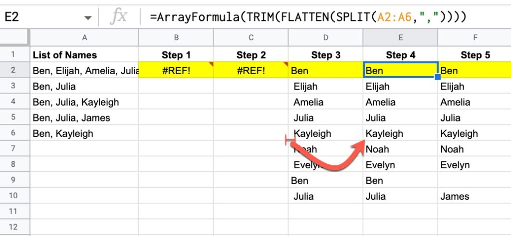
The TRIM function is used in step 4 to remove the leading spaces that were introduced by the earlier SPLIT function.
Read more about this specific example: How To Get A Unique List Of Items From A Column With Grouped Words.
Non-Formula Solution: Trim Whitespace With the Data Cleanup Tool
As an alternative to the TRIM function, you can use the Data Cleanup tool to remove unnecessary spaces. Here’s how it works:
Step 1: Highlight the range of data with whitespace issues.
Step 2: Click on the menu:
Data > Data cleanup > Trim whitespace
This will remove all extraneous whitespace in front of or at the end of words, as well as remove whitespace between words to leave only a single space.
TRIM Function Template
Click here to open a view-only copy >>
Feel free to make a copy: File > Make a copy…
If you can’t access the template, it might be because of your organization’s Google Workspace settings.
In this case, right-click the link to open it in an Incognito window to view it.
It’s part of the Text family of functions in Google Sheets. You can read about it in the Google Documentation.