How To Alternate Colors In Google Sheets

In this post, you’ll learn how to alternate colors in Google Sheets and add row or column banding to your data tables.

Here’s an example of alternating row bands applied to a checklist in Google Sheets:

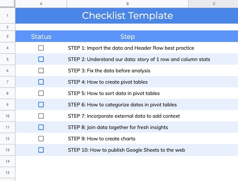
How To Alternate Colors In Google Sheets Rows

It’s super easy to add alternating row colors in Google Sheets.

Step 1:

Highlight your data table.

Step 2:

Go to Format > Alternating colors

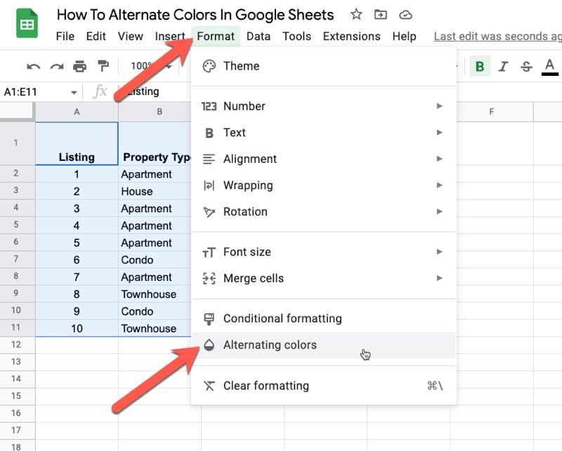
Step 3:

Select one of the default styles and click Done:

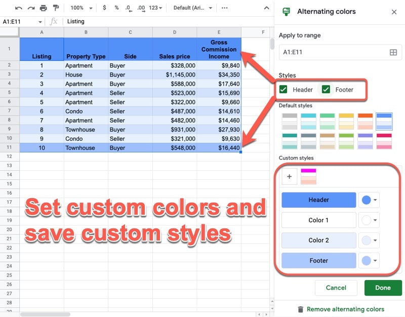
Custom Colors And Styles

There are two checkboxes in the alternating colors sidebar, which allow you to toggle headers and footers on or off. If you check them, you can set a different color for the headers and footers.

You can also set custom colors under the default styles and even save your color scheme as a custom style with the big plus button.

Dynamic Alternating Rows

How do you apply alternate colors in Google Sheets if your table is dynamic and changes size?

Unfortunately, you can’t use the alternating rows tool because it gets applied to a static range. The alternating color bands are left in place whether there is data or not.

But the good news is that you can use regular conditional formatting to achieve the dynamic alternating colors.

Highlight your data range, open the conditional formatting sidebar, and set the custom formula rule to:

Notice the $ sign in front of the A, so that the conditional formatting is applied to the whole row.

Also, this rule is operating on a range that starts from cell B16 (see the GIF above). You’ll want to change this to match the top-left cell of your range.

This formula works by checking that the row is an odd-numbered row AND not blank in column B, i.e. the row has data.

If the row is blank in column B, then the conditional formatting is not applied.

This technique could be adapted to columns by switching the ROW function to a COLUMN function.

How To Alternate Colors In Google Sheets Columns

Unfortunately, there is no equivalent alternating colors option that works on columns. However, since it’s much less common to do this, perhaps that’s no great loss.

But, in case you want to color columns with alternating colors, here’s how:

Step 1:

Highlight your data table.

Step 2:

Go to Format > Conditional formatting

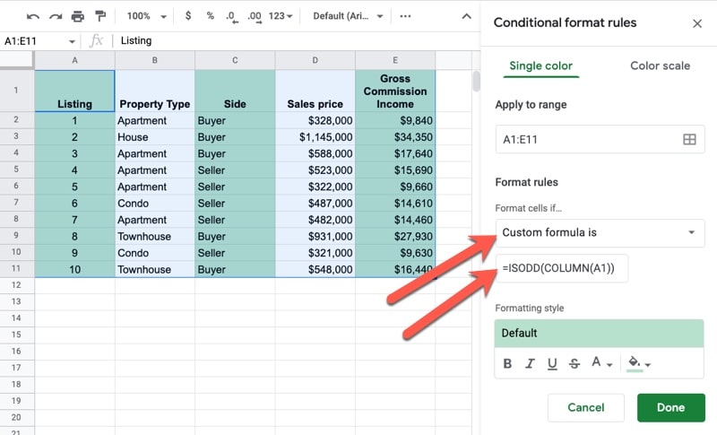
Step 3:

Set the format rule to “Custom formula is”

Step 4:

Enter this custom formula, using the ISODD function and the COLUMN function, if you want the color to start in column A:

Alternatively, use this formula with ISEVEN to start the colors from column B:

Step 5:

Set the formatting style and click Done.

See Also

How To Make a Table in Google Sheets, and Make It Look Great