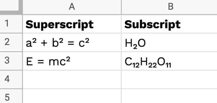
In this tutorial, you’ll learn how to add subscript or superscript characters in Google Sheets.
Continue reading How To Add Subscript and Superscript In Google Sheets
Educator and Google Developer Expert. Helping you navigate the world of spreadsheets & AI.
In this tutorial, you’ll learn how to add subscript or superscript characters in Google Sheets.
Continue reading How To Add Subscript and Superscript In Google Sheets
Conditional formatting is a super useful technique for formatting cells in your Google Sheets based on whether they meet certain conditions.
In this post, you’ll learn how to apply conditional formatting across an entire row of data in Google Sheets.
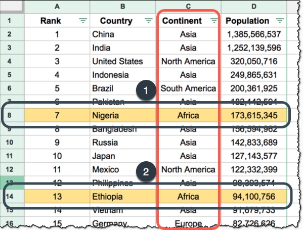
For example, if the continent is “Africa” in column C, you can apply the background formatting to the entire row (as shown by 1 and 2):
A template with all these examples is available at the end of this post.
Continue reading How To Apply Conditional Formatting Across An Entire Row In Google Sheets
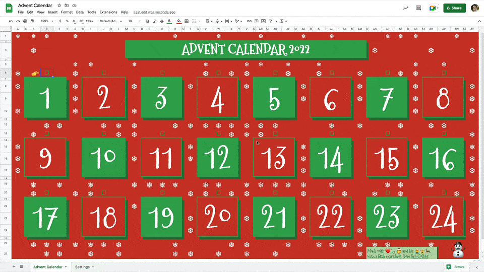
This year, I created a Google Sheets Advent Calendar, which you can see in action here:
It was a fun project with some interesting techniques, which are explored below.
You could easily modify it for your own example, or use these techniques in different scenarios.
Plus, if you’re too cheap to buy a physical advent calendar, this lets you enjoy the fun of opening a door each day to reveal something, but for free!
Continue reading Google Sheets Advent Calendar
This is a guest post from Josh Cottrell-Schloemer.
Google Sheets is an incredibly powerful spreadsheet tool for pulling, processing, and presenting data. But many people don’t realize that you can also use it to build interactive dashboards.
With a bit of creativity we can go from this:
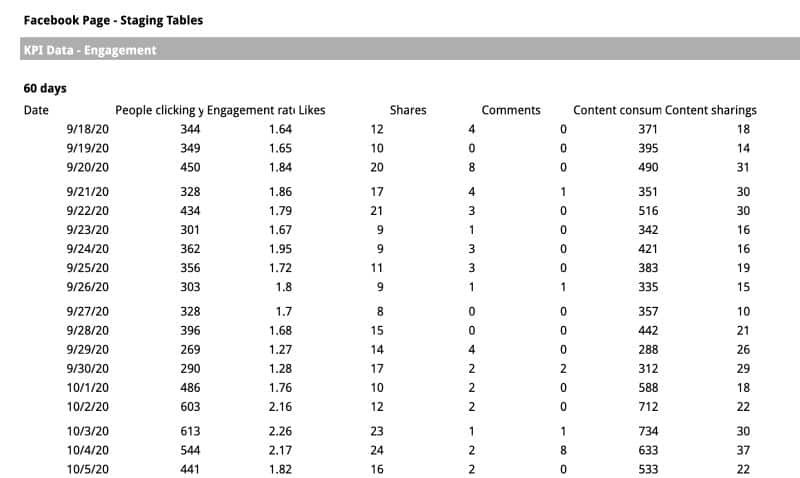
To this:
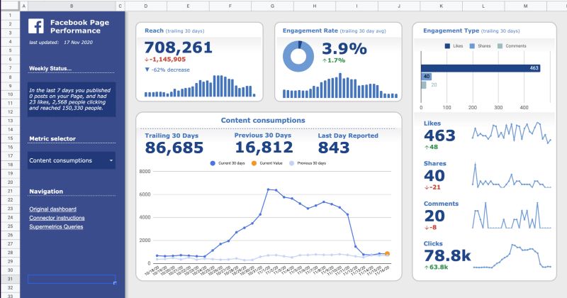
The skills to build this type of dashboard aren’t difficult to learn and you can get started with a basic knowledge of Google Sheets.
Here’s a walkthrough of the dashboard shown above:
Continue reading Making Google Sheets look less like… Google Sheets
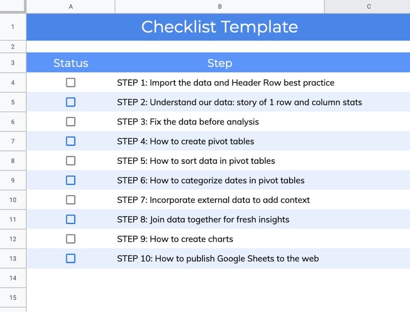
In this post, you’ll learn how to alternate colors in Google Sheets and add row or column banding to your data tables.
Here’s an example of alternating row bands applied to a checklist in Google Sheets: