Google Sheets COUNTIF Function

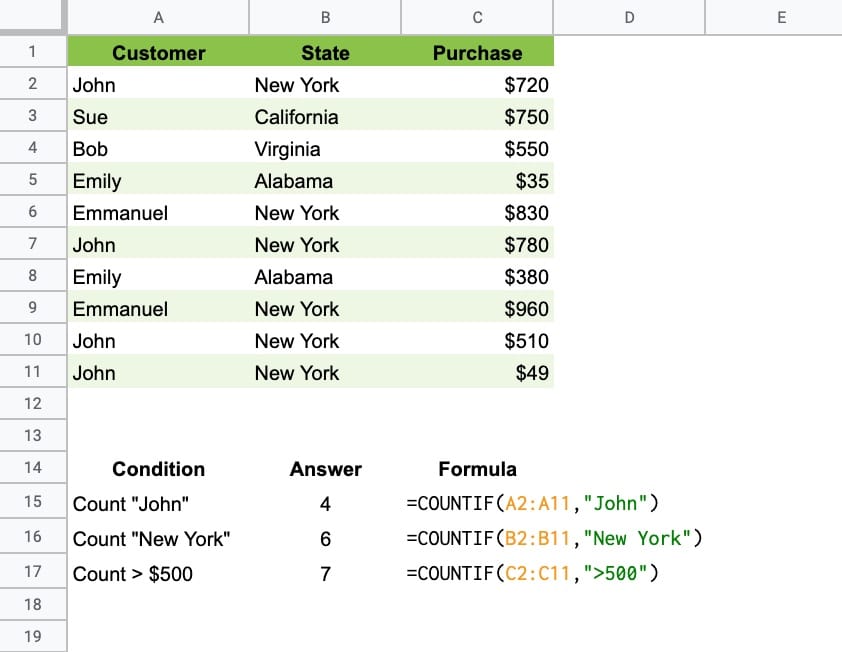
The Google Sheets COUNTIF function is used to count items in a range that match a given condition.

For example, consider the following dataset of customer sales:

This formula counts how many times “John” is found in the range:

This one counts how many times “New York” occurs:

And this one counts how many sales are over $500:

COUNTIF Function Syntax

It takes 2 arguments:

• range
• criterion

The range is the data that you want to count across.

The criterion is the test you want to apply. If you want to apply multiple tests for counting, then you need to use the COUNTIFS function.

Think of the COUNTIF function as the love child of the IF function and COUNT function.

It’s part of the Math family of functions in Google Sheets.

COUNTIF Function Notes

Text Criterion

Text criterion must be enclosed by quotes:

This formula will count all cells that are equal to the word Apartment.

Numeric Criterion

Exact matches with numeric values do not require quotes:

This counts all cells with a value of 500.

Conditional Tests

Logical operators are used to create conditional tests:

• > greater than
• >= greater than or equal to
• < less than
• <= less than or equal to
• = equal to
• <> not equal to

They must be enclosed with double quotes:

This counts all cells with values greater than 500.

Case Insensitive

COUNTIF is case insensitive, so these two formulas will produce the same result:

Counting Blanks and Non Blanks

To count blank cells in a range, use empty double quotes:

To count non-blank cells in a range, use the not-equal logical operator “<>“:

Reference another cell

The criterion for COUNTIF function can be contained in a different cell and referenced by the COUNTIF formula:

If you want to use a logical operator, then it must still be enclosed in double-quotes. Use an ampersand to combine with the reference cell:

Using Wildcards with COUNTIF

COUNTIF Google Sheets supports three wildcards, *, ?, and ~.

The star * matches zero or more characters.

The question mark ? matches exactly one character.

The tilde ~ is an escape character that lets you search for a * or ?, instead of using them as wildcards.

Let’s see some examples:

Star wildcard

The star wildcard can go in front of, at the end of, or at both ends of your search string. This formula:

will count any values containing house, e.g. house, townhouse, big house, house for sale, etc.

Wildcards can be used with reference cells too:

Question mark wildcard

This formula:

will match any string with 3 characters where the first character is “J” and the last character is “n”, e.g. Jon, Jen, and Jan (as well as JXn, JZn, J7n, etc.).

Tilde Escape wildcard

The Tilde ~ is used when you want to search for the wildcard characters themselves e.g. * and ?

counts all cells containing Yes*, and

counts all cells containing Yes?

COUNTIF Template

All of the examples above are available in the following template.

Click here to open a view-only copy >>

Feel free to make a copy: File > Make a copy…

If you can’t access the template, it might be because of your organization’s Google Workspace settings. If you right-click the link and open it in an Incognito window you’ll be able to see it.

You can also read about it in the Google Documentation.