The SEQUENCE function is a useful function in Google Sheets. It’s a powerful way to generate numbered lists.
SEQUENCE Function Syntax
=SEQUENCE(rows, columns, start, step)As arguments for the SEQUENCE function, you specify 1) the number of rows, 2) the number of columns, 3) a start value, and 4) a step size.
Arguments 2, 3, and 4 are optional. However, if you want to set them you need to include the previous ones (e.g. if you want to set a step size in argument 4, then you need to set 1, 2, and 3 as well).
Keep this order in mind as you look through the examples below and you’ll soon understand how the function works.
1. Ascending list of numbers
=SEQUENCE(5)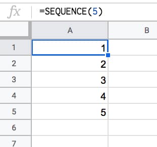
2. Horizontal list of numbers
Set the row count to 1 and the column count to however many numbers you want e.g. 5:
=SEQUENCE(1,5)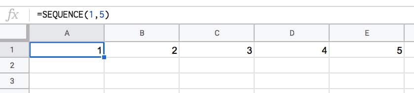
3. Two-dimensional array of numbers
Set both row and number values:
=SEQUENCE(5,5)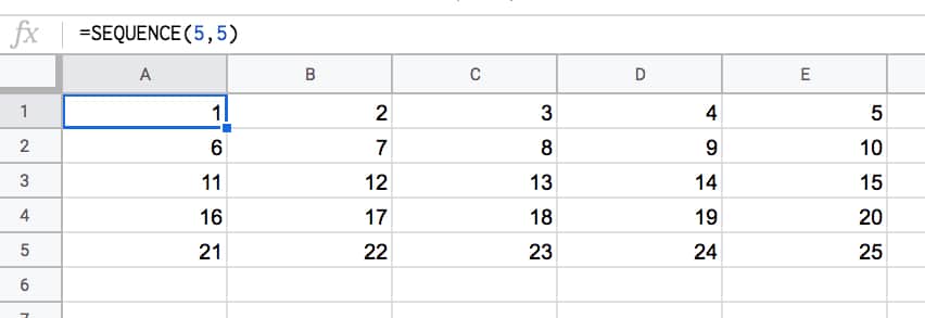
4. Start from a specific value
Set the third argument to the value you want to start from e.g. 100:
=SEQUENCE(5,1,100)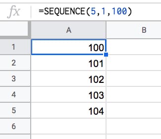
5. Use a custom step
Set the fourth argument to the size of the step you want to use, e.g. 10:
=SEQUENCE(5,1,1,10)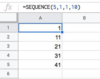
6. Descending numbers
Set the fourth argument to -1 to count down:
=SEQUENCE(5,1,5,-1)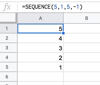
7. Negative numbers
Set the start value to a negative number and/or count down with negative step:
=SEQUENCE(5,1,-1,-1)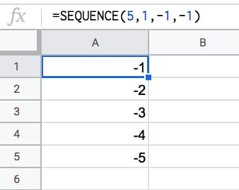
8. Dates
Dates are stored as numbers in spreadsheets, so you can use them inside the SEQUENCE function. You need to format the column as dates:
=SEQUENCE(5,1,TODAY(),1)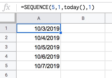
9. Decimal numbers
Unfortunately you can’t set decimal counts directly inside the SEQUENCE function, so you have to combine with an Array Formula e.g.
=ArrayFormula( SEQUENCE(5,1,10,1) / 10 )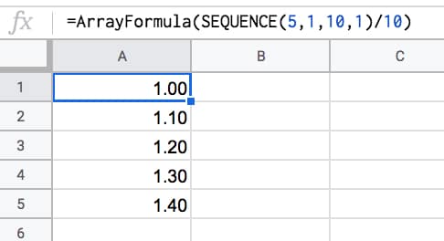
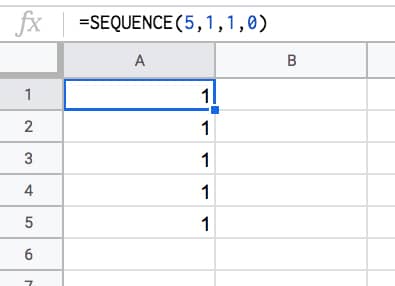
10. Constant numbers
You’re free to set the step value to 0 if you want an array of constant numbers:
11. Monthly sequences
Start with this formula in cell A1, which gives the numbers 1 to 12 in a column:
=SEQUENCE(12)In the adjacent column, use this DATE function to create the first day of each month (formula needs to be copied down all 12 rows):
=DATE(2021,A1,1)This can be turned into an Array Formula in the adjacent column, so that a single formula, in cell C1, outputs all 12 dates:
=ArrayFormula(DATE(2021,A1:A12,1))Finally, the original SEQUENCE formula can be nested in place of the range reference, using this formula in cell D1:
=ArrayFormula(DATE(2021,SEQUENCE(12),1))This single formula gives the output:
1/1/2021
2/1/2021
.
.
.
12/1/2021
It’s an elegant way to create a monthly list. It’s not dependent on any other input cells either (columns A, B, C are working columns in this example).
With this formula, you can easily change all the dates, e.g. to 2022.
Building in steps like this a great example of the Onion Method, which I advocate for complex formulas.
12. Text and Emoji sequences
You can use a clever trick to set the SEQUENCE output to a blank string using the TEXT function. Then you can append on a text value or an emoji or whatever string you want to create a text list.
For example, this repeats the name “Ben Collins” one hundred times in a column:
=ArrayFormula(TEXT(SEQUENCE(100,1,1,1),"")&"Ben Collins")And, by using the CHAR function, you can also make emoji lists. For example, here’s a 10 by 10 grid of tacos:
=ArrayFormula(TEXT(SEQUENCE(10,10,1,1),"")&CHAR(127790))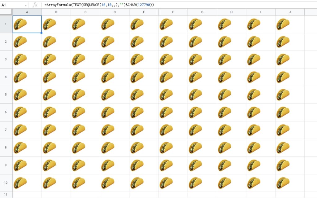
13. Lists Of Grouped Numbers
Suppose we’re organizing an event and we want to group our 20 participants into groups of 5.
Start with the standard SEQUENCE function to output a numbered list from 1 to 20:
=SEQUENCE(20)Next, divide by 5:
=SEQUENCE(20)/5This gives a single output, 0.2, so we need to wrap it with an array formula to get the full column output:
=ArrayFormula(SEQUENCE(20)/5)Finally, we add ROUNDUP to create the groups shown in the image above:
=ArrayFormula(ROUNDUP(SEQUENCE(20)/5))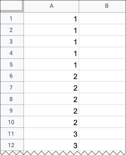
14. Repeating Sequence
To create a repeating sequence 1,2,3,1,2,3,1,2,3,etc. use the SEQUENCE function in combination with the MOD function:
=ArrayFormula(MOD(SEQUENCE(100,1,0),3)+1)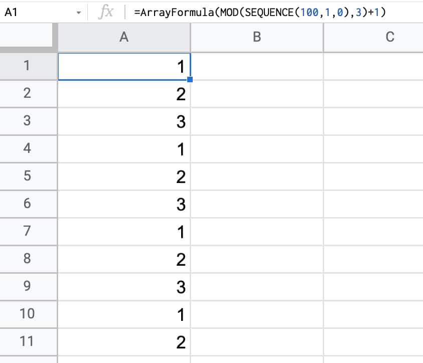
Have you got any examples of using the SEQUENCE function?
Hi Ben!
Always loved your way of creativity. You see all possibilities in a single function.
Please see the first 50 Fibonacci numbers
=index(((1+5^(1/2))^SEQUENCE(50)-(1-5^(1/2))^SEQUENCE(50))/(2^SEQUENCE(50)*5^(1/2)))Love it! Great work, Max!
1. Wrap the SEQUENCE in an ARRAYFORMULA(ROUNDUP & a divide operation to make multiples of each number in the list, e.g. =ARRAYFORUMLA(ROUNDUP(SEQUENCE(9,1,1)/3)) generates a column vector {1;1;1;2;2;2;3;3;3}
2. Feed a SEQUENCE starting at 65 into an ARRAYFORMULA(CHAR to create a sequence of letters (because CHAR(65)=”A”), e.g. =ARRAYFORMULA(CHAR(SEQUENCE(1,9,65))) generates a row vector {A,B,C,D,E,F,G,H,I}
3. Concatenate row & column vectors generated with SEQUENCE using ‘&’ within the ARRAYFORUMLA to generate grids containing all the possible combinations (e.g. concatenating the above two examples generates an 9×9 grid starting at 1A & ending at 3I)
Very nice! I like the row vector of letters. Thanks for sharing.
Cheers,
Ben
Hi Ben,
Could you do an article about non-linear and looping sequences?
For example I’m stuck trying trying make this simple sequence for many rows: 1,2,3,5,1,2,3,5,1,2,3,5
Hope I’m not treading on anyone’s toes here, but I’d approach it like this (e.g. for 10 loops): =ARRAYFORMULA(FLATTEN({1,2,3,5}&LEFT(A1:A10,0)))
N.B. Using 0 as the second argument of LEFT returns an empty string; within an ARRAYFORMULA empty arrays can be made this way. The column of cells referred to in the LEFT can be anywhere on the sheet; it is the number of cells in the column range that controls the number of loops.
Hi Lucas,
There are several ways of creating non-linear sequences. One method is to use Query to filter out non wanted values.
Example:
=ArrayFormula(QUERY(
MOD(SEQUENCE(50),6),
"Select Col1
Where Col1 != 0
AND Col1 != 4 ",0 )
)
Thanks, Ben! Especially for monthly sequences.
Is there any way to upgrade the formula when I want every month for example three times?
I mean
1/7/2021
1/7/2021
1/7/2021
1/8/2021
1/8/2021
1/8/2021
and so on till the end of the next year.
Thank you.
Milan
This generates a sequence of 3’s for the 12 months of the year
=ArrayFormula(“1/”&ROUNDUP(SEQUENCE(36)/3)&”/2021”)
Very nice and helpful. 🙂
HI BEN,
How can we make a list that starts with a constant, the output required :
AB-1
AB-2
AB-3
….
I tried =CONCATENATE(“AB-“,SEQUENCE(10,1,1,1))
got AB-12345678910
the only solution for me now is to make a column with sequence
and then concatenate to another column.
can you have a solution to make it in one step
=SEQUENCE(10,1,1,1) | =CONCATENATE(“AB-“,T12)
1 | AB-1
2 |AB-2
3…..
Akram wrap it with an array formula, using the TEXT function to concatenate.
=ARRAYFORMULA(TEXT(SEQUENCE(10;1;1;1);”\A\B\-0″))
=ArrayFormula(“AB-“&sequence(10))
THANK YOU! my brain was dead this morning and I couldn’t rub the sticks together.
=ARRAYFORMULA(“AB-“&SEQUENCE(5,1,1,1))
Ignore my previous comment.
Ben,
Is there a way to use the sequence where I have a spreadsheet with the layout below that the Column A represents the equipment ID and column B is the sequence of the orders to be ran. The first row of each pieces of equipment is empty and could house a formula but new orders are added and old ones taken out daily. I would just like to be able to sequence automatically.
Thanks
F102
F102 1
F102 2
F102 3
F104
F104 1
F104 2
F104 3
F104 4
F105
F105 1
F105 2
Hi Jim, did you find a way to do this? I have the same challenge!
Im also trying to find a way to do this.
Trying to take the difference between two numbers which we are abbreviating as years. For example,
we enter in 50 60 in a cell. I want to have this output
1950 1951 1952 1953 1954 1955 1956 1957 1958 1959 1960.
First I was splitting the cell into two columns then adding 1900 to each number to change this to the correct year. We don’t care about any years in the 2000’s only the 1900s.
Was then attempting to use the sequence function to only show the years between the two values but I can’t seem to figure how to do this.
Hey Darren,
Not sure exactly what you’re trying to do, but these two sequence functions will give you that output you want:
In a column:
=SEQUENCE(10,1,1950,1)As a row:
=SEQUENCE(1,10,1950,1)Hope this helps!
Ben
I have to create variable length sequences from a column along its rows.
Eg- Suppose the column is as below
2
4
3
I want to create a sequence like this
2 | 1 | 2
4 | 1 | 2 | 3 | 4
3 | 1 | 2 | 3
I’m able to create a single sequence using the SEQUENCE function but to spread it over the entire column, I’m not able to use the ARRAYFORMULA correctly.
If I write ARRAYFORMULA(SEQUENCE(A1:A3)), it gives me a column of three ones.
Hi, did you find a solution?
Hey Dhruv, let’s assume 2, 4, and 3 are in cells: A1, A2, A3
In B1, put =SEQUENCE(1, A1, 1, 1)
Row Count = 1
Column Width = A1 (This is your starting number, which will work as how many columns you have if you’re counting up to it)
Start Value = 1
Increase by = 1
Hi,
I’m trying to create a serial numbers, including the year and month from a date field in the sheet.
Something like:
22-06-001
22-06-002
22-06-003
22-07-001
22-07-002
etc.
Thanks in advance!
Hy
How i can create a formula for a results:
1 of 4
2 of 4
3 of 4
4 of 4
if there are duplicate numbers in a column
Hi Sergiu,
You can use either of these formulas to create lists like that:
=ArrayFormula(SEQUENCE(4)&" of 4")or, with the new lambda byrow function:
=BYROW(SEQUENCE(4),LAMBDA(row,row&" of "&4))Cheers,
Ben
Surely the most compact form would be =ARRAYFORMULA(SEQUENCE(4)&” of 4″) – you don’t need to create a {4;4;4;4} array with the second SEQUENCE as you can just ‘&’ the constant “of 4″ to each element of the {1;2;3;4} array generated by the first SEQUENCE…
Or if you wanted to LAMBDAify it:
=ARRAYFORMULA(LAMBDA(n,SEQUENCE(n)&” of “&n)(4))
Yes, agreed! Thanks for sharing. I’ve updated my answer.
P.S. Nice work with the lambda only solution 🙂
Hi Ben. May i know if i can add the text in front of the number and keep them running like AA001/2023, AA002/2023, AA003/2023 and so on. Your help is greatly appreciated. Thank you so much
Hi Ben – very helpful post (as is your website in general).
Do you know if it is possible to offset the starting position of a Sequence (or other array) formula?
Here’s my issue:
I have two columns that represent current and target values (range is 1:9, and current value will always be <= target value). I need to create a sequence across columns that is equal to target minus current plus 1, and have the resulting array begin under the column equal to the starting number of the sequence.
So for example, if current value = 4 and target value = 6, the resulting sequence should be 4, 5, 6, and it should begin under the 6th column.
Here's the set up:
Column: Column A | Column B | Column C
Header: Current Stage | Target Stage | Sequence Formula
Example with traditional sequence formula:
4 | 6 | 4 | 5 | 6
What I am trying to create (using example above):
Column: A | B | C | D | E | F | G | H | I | J | K
Header: Current | Target | 1 | 2 | 3 | 4 | 5 | 6 | 7 | 8 | 9
Row 2: 4 | 6 | * | | | 4 | 5 | 6 | …
*where Sequence formula lives
Formula in cell C2: =SEQUENCE(1,B1-A1+1,A1,1)
I am trying to get the result of [4|5|6] to start under column F (header = 4).
I’ve tried variations of the Offset and IF functions, but am wondering if I’m either missing something obvious or what I’m trying to do isn’t possible. Any help would be highly appreciated!
Thanks,
Scott
Update: I managed to get it to work with a simple IF/AND formula. Would still be interesting to see if an Offset/Sequence combination could work, though.
=IF(AND($A2=C$1,$B2""),C$1,"")This reply does not makes sense. It also gives a parse error. It seems that either some serious mistake was committed or the request was not understood
I’m trying to build a column that lists dates in a sequence of 8, and found this thread. Admittedly, I’m somewhat inexperienced but have attempted to derive a solution based on some of the info and replies here.
Can anyone help figure out the necessary instructions to achieve a sequential order of dates, with a sequence of 8 of the same date? I need to create a years worth of dates in this order, with 8 rows dated per day of 2023.
01/01/2023
01/01/2023
01/01/2023
01/01/2023
01/01/2023
01/01/2023
01/01/2023
01/01/2023
01/02/2023
01/02/2023
01/02/2023
01/02/2023
01/02/2023
01/02/2023
01/02/2023
01/02/2023
Is there a way to use SEQUENCE to generate a list of values that will be in one Cell only. For example, something like “Col” & SEQUENCE(5) &”, “. I will use this output in a QUERY command, so I need everything in one cell only
Hi there, Use the JOIN function to combine the outputs of the SEQUENCE function to achieve this.
I need to make a simple SEQUENCE in column A, but as long as I have any data in column B. How can I do it? Thank you for your advice!
Short video explanation: https://drive.google.com/file/d/1IrvpyPv5BHlpil7afKjwx4aGn0PEahj2/view?usp=drivesdk
You can use this in A1 and then copy it down to the whole column A:
=IF(B1″”, ROW()-1, “”)
Or if you want to use SEQUENCE you can try this:
=ARRAYFORMULA(IF(B:B””,SEQUENCE(COUNTA(FILTER(B:B,B:B””))),))
I hope it helps you!
I tried to use Bycol in a cell A5, and sequence in a different cell D1.
Bycol merges into sequence. one should generate error.
I have values of A1=1,A2=2. Bycol uses, average value and the range is A1:2. So, it expands to any columns.
In this case, I have used sequence in B1 cell to list 50. Now, surprisingly, the Bycol merges into sequence. So, B3 cell, I am getting average of B1 and B2. So, B3=1.5 instead of 3. It is a bug with the sequence or Bycol. I expect, that Bycol should give an error.
Hi! I have a sheet of rows with 4 columns but the rows are all out of order.
UniqueID| String | PrevString | NextString
I’m trying to figure out how to get the rows sorted in the right sequential order based on knowing what is the “PrevString” that comes before “String” and the “NextString” that follows it.
“PrevString” and “NextString” values all appear in the “String” row once.
Any ideas?
I need help with making this kind of sequence:
1-2000
2001-4000
4001-6000
6001-8000
8001-10000
ect…
in 2000’s I need to make it until 630k
please help thank you
Hi,
I Want to
This 611989864546
become
6 1 1 9 8 9 8 6 4 5 4 6 This
which formula I can use.
Hello ,
So I’m trying to get my google sheets to count like this.
1101-1
1101-2
1101-3
1101-4
1102-1
1102-2
1102-3
1102-4
and so on,
how would i do this?
I would reconfigure Maksim’s brilliant function with =let() as follows:
=let(q,5^0.5,s,sequence(A2),index(((1+q)^s-(1-q)^s)/((2^s)*q)))
I am trying to repeat a random list of numbers which changes daily.
so in day 1 50 numbers day 2 75 day 3 63 etc,,,
I have tried isblank formulas so once it gets to the end of the list loops back until row 200 is reached and i have also tried the =ARRAYFORMULA(INDEX(‘ops sheet details’!R3:R,MOD(SEQUENCE(220)-1,COUNTA(‘ops sheet details’!R3:R))+1))
However i can not get this to repeat the number list, any suggestions?