Behold the Google Sheets Formula Clock, a working analog clock built with a single Google Sheets formula:
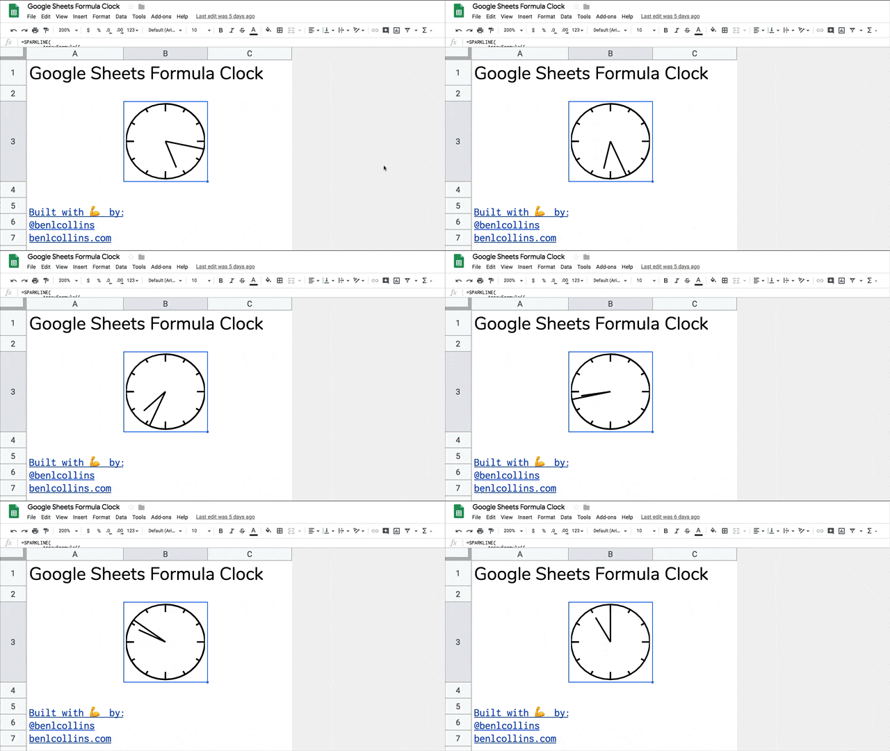
It’s a working analog clock built with a single Google Sheets formula.
That’s right, just a single formula. No Apps Script code. No widgets. No hidden add-ons.
Just a plain ol’ formula in Google Sheets!
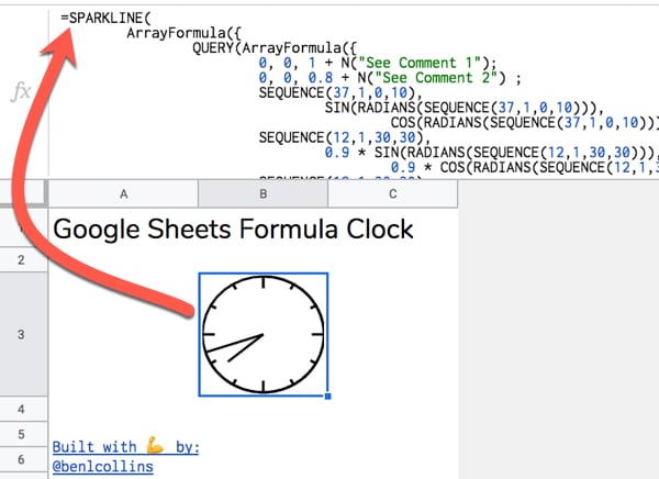
Google Sheets Formula Clock Template
Click here to open the Google Sheets Formula Clock Template
(Click to open the template. Feel free to create your own copy through the File menu: File > Make a copy...)
It might take a moment to update to the current time.
Part 1: Build your own Google Sheets Formula Clock
Step 1
Open a blank Google Sheet or create a new Google Sheet
(Pro-tip: type sheet.new into your browser address bar to do this instantly)
Step 2
Copy the Google Sheets Formula Clock formula below and paste it into the formula bar for cell A1 of your new Sheet:
=SPARKLINE(

        ArrayFormula({

                QUERY(ArrayFormula({

                        0, 0, 1 + N("See Comment 1");

                        0, 0, 0.8 + N("See Comment 2") ;

                        SEQUENCE(37,1,0,10),

                                SIN(RADIANS(SEQUENCE(37,1,0,10))),

                                        COS(RADIANS(SEQUENCE(37,1,0,10))) + N("See Comment 3") ;

                        SEQUENCE(12,1,30,30),

                                0.9 * SIN(RADIANS(SEQUENCE(12,1,30,30))),

                                        0.9 * COS(RADIANS(SEQUENCE(12,1,30,30))) + N("See Comment 4") ;

                        SEQUENCE(12,1,30,30),

                                SIN(RADIANS(SEQUENCE(12,1,30,30))),

                                        COS(RADIANS(SEQUENCE(12,1,30,30))) + N("See Comment 5") ;

                        SEQUENCE(4,1,90,90),

                                0.8 * SIN(RADIANS(SEQUENCE(4,1,90,90))),

                                        0.8 * COS(RADIANS(SEQUENCE(4,1,90,90))) + N("See Comment 6") ;

                        SEQUENCE(4,1,90,90),

                                SIN(RADIANS(SEQUENCE(4,1,90,90))),

                                        COS(RADIANS(SEQUENCE(4,1,90,90))) + N("See Comment 7")

                        }),

                        "SELECT Col2, Col3 ORDER BY Col1",

                        0  + N("See Comment 8")

                ) ;

                IF(

                        MINUTE(NOW()) = 0,

                        0,

                        SIN(RADIANS(SEQUENCE(MINUTE(NOW())/60*360,1,1,1)))

                ),

                IF(

                        MINUTE(NOW())=0,

                        1,

                        COS(RADIANS(SEQUENCE(MINUTE(NOW())/60*360,1,1,1)))

                )  + N("See Comment 9");

                0, 0 + N("See Comment 10") ;

                0.75 * SIN(RADIANS((MOD(HOUR(NOW()),12)/12 * 360) + MINUTE(NOW())/60 * 30)),

                        0.75 * COS(RADIANS((MOD(HOUR(NOW()),12)/12 * 360) + MINUTE(NOW())/60 * 30)) + N("See Comment 11")

        }),

        {"linewidth",2 + N("See Comment 12")

        + N("

                Comments:

                1: Initial (0,1) coordinate at top of circle. Extra 0 included for sort.

                2: Coordinates to create mark at 12 o'clock.

                3: Coordinates to draw initial circle. Joins markers every 10 degrees starting from 0 at top of circle, e.g. 0, 10, 20, 30,...360

                4: Sequence of coordinates every 30 degrees to create small markers for hours 1, 2, 4, 5, 7, 8, 10, 11

                5: Sequence of coordinates to connect the 30 degree small markers. Needed to place them correctly on circle.

                6: Sequence of coordinates every 90 degrees to create large markers for hours 12, 3, 6, 9

                7: Sequence of coordinates to connect the 90 degree large markers. Needed to place them correctly on circle.

                8: QUERY function used to sort the circle data by the degrees column, then select just the (x,y) coordinate columns (numbers 2 and 3) to use.

                9: Coordinates to create the minute hand. Includes an IF statement to avoid an error when the minute hand arrives at the 12 mark.

                10: Coordinates to return to centre of clock at (0,0) after minute hand, to be ready to draw hour hand.

                11: Coordinates to create the hour hand.

                12: Set linewidth of the Sparkline to 2.

                .

                .

                Google Sheets Formula Clock

                June 2019

                Created by Ben Collins, Google Developer Expert and Founder of The Collins School Of Data

                Website: benlcollins.com

                Twitter: @benlcollins

        ")}

)
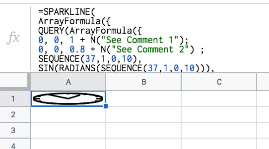
Initially it will look like this:
Step 3
Make row 1 wider by hovering between rows 1 and 2 and using the grab hand to drag the row boundary down. Make the cell wide enough to create a circle:
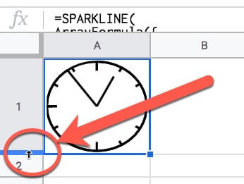
Step 4
This is the step that makes the clock tick!
Under File > Spreadsheet settings set the spreadsheet calculation settings to be “On change and every minute”, like so:
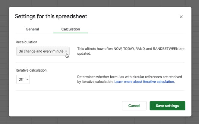
This ensures that the NOW function is refreshed every minute, so our clock hands move around the circle. That’s it!
You should see the hands of your clock moving around the face.
Tick-tock! Tick-tock!
Part 2: How Does It Work?
So there are a few things going on here.
We need a way to get the current hour and minute values and have them update automatically.
Then somehow we need to draw a clock face with hands using…formulas?
Let’s run through the building blocks…
Create A Circle With The Sparkline Function
The SPARKLINE function is used to create miniature charts inside a single cell. That’s its modus operandi.
However, we can also supply it with a range of x- and y-coordinates to create 2-d shapes, like a circle for example.
Use the following five steps to create a circle with a sparkline:
1) Start with this function in cell A1:
= SEQUENCE ( 37, 1, 0, 10 )The SEQUENCE function creates 37 rows in a single column, starting from 0 and increasing in increments of 10 each.
I.e. it outputs a column of numbers representing every 10 degrees of a circle, up to 360 degrees.
2) In column B, we add this Array Formula in cell B1:
= ArrayFormula ( SIN ( RADIANS ( $A$1:$A$37 ) ) )3) And in column C, this one in cell C1:
= ArrayFormula ( COS ( RADIANS ( $A$1:$A$37 ) ) )Columns B and C now give you the coordinates of a circle.
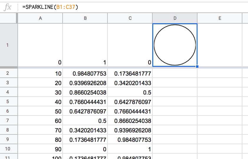
4) Let’s plug them into the SPARKLINE function in cell D1 with this function:
= SPARKLINE ( B:C )5) Lastly, make row 1 wider to show the circle.
Boom!
The SPARKLINE function draws a circle for us:
Then, we need to create a time that automatically updates every minute. Thankfully that’s relatively easy to do with the NOW function:
NOW Function + Spreadsheet Settings
(Feel free to type these formulas in to the side of your sparkline workings in column B, C and D.)
= NOW()The NOW Function in Google Sheets outputs a timestamp with a time to the nearest second. It’s a volatile function, which means it recalculates every time a change is made to the Sheet. In other words, it gives a new timestamp.
Per the Step 4 in Part 1 above, we can set the Sheet to update every minute, so the NOW function updates every minute.
Get The MINUTE And HOUR From NOW
It’s relatively easy to extract the minute and hour from the timestamp, with these two functions:
= MINUTE( NOW() )and
= HOUR ( NOW() )We need to convert these to degrees on a circle to show how far round the hands have gone.
The formulas become:
= MINUTE( NOW() ) / 60 * 360and
= MOD( HOUR( NOW() ), 12 ) / 12 * 360respectively.
Later we’ll need to convert these to RADIANS and then into coordinates for the sparkline function.
That’s the mechanics of the clock-tick-tock part, but we still need to add them to our sparkline clock.
Add The Clock Hands
The middle of our circle is represented by the coordinates (0,0).
Currently, our sparkline has positioned us at the 12 o’clock position, represented by (0,1).
To add the minute hand, we need to draw another arc around the circle to travel around the edge of the circle to the current minute value, e.g. if it’s half past the hour then we need to draw another half circle to position ourselves at the bottom of the circle.
Then we can simply draw a line back to the center of the circle, and that’s our minute hand!
So, add this function to cell B38:
=ArrayFormula( SIN ( RADIANS ( SEQUENCE ( MINUTE ( NOW( ) ) / 60 * 360 , 1 , 1 , 1 ) ) ) )And add this one to cell C38:
=ArrayFormula( COS ( RADIANS ( SEQUENCE ( MINUTE ( NOW( ) ) / 60 * 360 , 1 , 1 , 1 ) ) ) )Essentially, what these two formulas are doing is working out how many degrees around the circle we need to go, and calculating the coordinates.
Finally, let’s return to the center of our circle, thereby drawing the minute hand.
In cell B398 put a 0.
In cell C398 put a 0.
They need to be on row 398 to give the array formula for the minutes enough space to expand (max 360 rows).
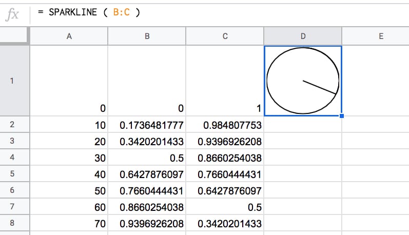
The “clock” now looks like this, and if you’ve set your spreadsheet to update every minute (see Step 4 in Part 1 above) then you’ll see this hand move around the clock.
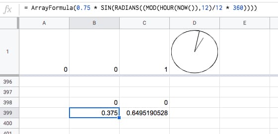
To add the hour hand, it’s a case of drawing a line from the centre coordinate (0,0) — where we are now — back out to the edge, again, going as far around the circle as needed to represent the current hour.
Add this formula to cell B399:
= 0.75 * SIN ( RADIANS ( ( MOD ( HOUR ( NOW( ) ) , 12 ) / 12 * 360 ) ) )And this formula to cell C399:
= 0.75 * COS ( RADIANS ( ( MOD ( HOUR ( NOW( ) ) , 12 ) / 12 * 360 ) ) )This adds the hour hand.
The 0.75 multiplier at the front of the formula shortens the hour hand a little to distinguish it from the second hand.
Boom!
Now you have a working clock:
Click here to view the template of this intermediary step.
Fix The Hour Issue
Unfortunately, in it’s current state, the formula breaks down at the top of the hour:
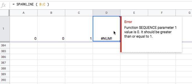
This is easily solved by wrapping the minute hand calculation with an IF statement to set it to zero at the top of the hour. This IF statement tests to see if the minute component of NOW is equal to zero and sets the value to 0 if it is, otherwise we just proceed with the full SEQUENCE function.
Change the formula in cell B38 to
=ArrayFormula( IF( MINUTE( NOW() ) = 0 , 0 , SIN( RADIANS( SEQUENCE( MINUTE( NOW() ) / 60*360 , 1 , 1 , 1 )))))and the formula in cell C38 to
=ArrayFormula( IF( MINUTE( NOW() ) = 0 , 0 , COS( RADIANS( SEQUENCE( MINUTE( NOW() ) / 60*360 , 1 , 1 , 1 )))))It won’t look any different but you’ll avoid that error when the minute hand goes past the hour mark.
This formula is demonstrated in tab 2 of the intermediary template.
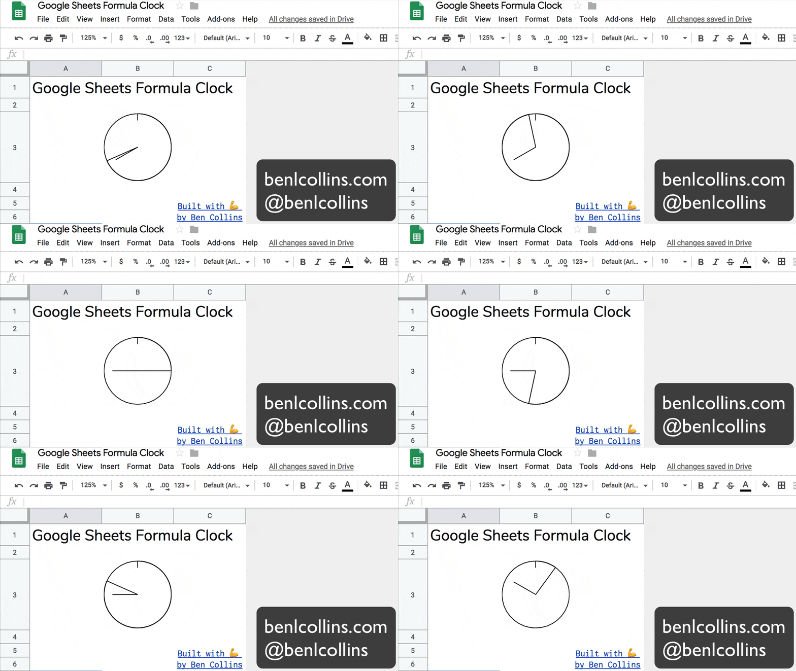
The clock will now look something like this:
So what’s left?
Improvements
You might consider the following improvements, but I’ll leave these as a challenge for you:
- Smoothing the hour hand, so it doesn’t jump in discrete steps from hour to hour but instead moves smoothly between the hours in proportion to the number of minutes passed. (See the GIF image at the start of this post.)
- Adding tick marks at each of the 12 hour marks around the clock face.
- Combining all the separate formulas into a single array formula. Hint: you need to make use of array literals with the constituent formulas.
- Add comments to explain the parts of the formula (see adding comments using the N function)
Implementing all of these is a little tricky, not the least because the formula gets rather long!
The best approach is to build in steps, employing the Onion Method technique to avoid frustrating errors.
Hickory, dickory, dock.
The mouse ran up the sparkline clock.
The sparkline clock struck one,
The mouse ran down,
Hickory, dickory, dock. 🐁 ⏱️
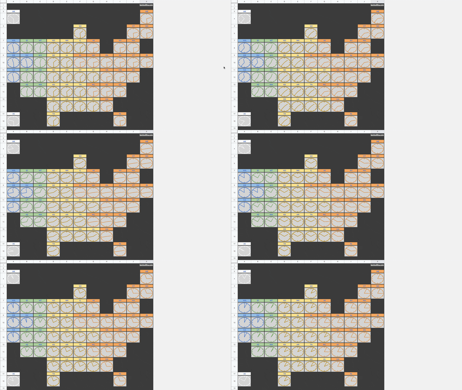
US Timezone Map
Combining many of these analog sparkline clocks onto a tile map, you can create this timezone map of the US:
Digital Clock?
See also this impressive digital clock built in Google Sheets by Robin Lord.
What Else Can You Draw With Sparklines?
Your imagination is the only limit with the sparkline function.
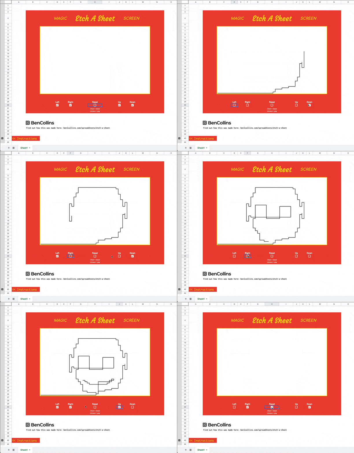
How about an Etch-A-Sketch clone built using a sparkline formula?
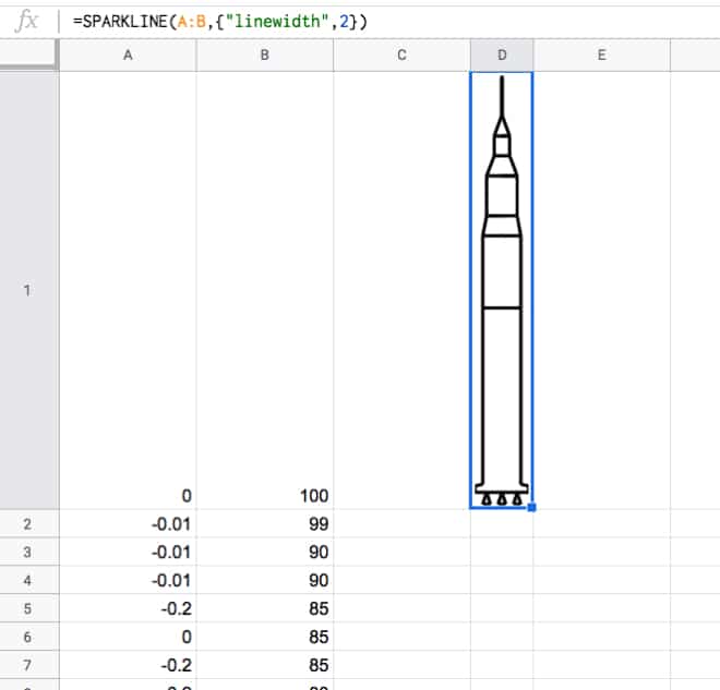
Or how about an outline of the Saturn V rocket?
Or a pie chart built with a single sparkline array formula?
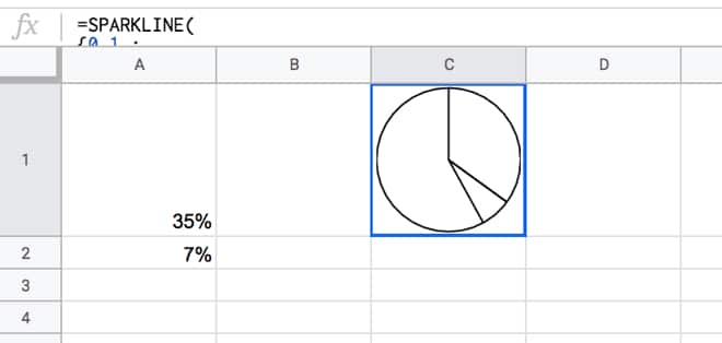
This pie chart actually inspired the analog clock…you can probably see why!

I am collecting my Jaws from the floor!!!!
and the formula in cell B39 to
=ArrayFormula( IF( MINUTE( NOW() ) = 0 , 0 , COS( RADIANS( SEQUENCE( MINUTE( NOW() ) / 60*360 , 1 , 1 , 1 )))))
Did you mean C39?
Good spot! I meant C38…have updated the post now 😉
Could you add a one-line pre-explanation of the SEQUENCE function, for those of us who’ve not encountered it before (and are now thinking of SO many ways to use it!). As little as:
=SEQUENCE (rows, columns, start, step)
Sure. I’ve added that 🙂
Ben, you’re either a genius or a lunatic. Or perhaps both.
Definitely not the former… so I guess the latter
Woah! Love this. I’m learning so much from you.
You’re welcome! Thanks for stopping by
Nice thing,
I want to configure live sql data base with Google spreadsheet, Is it possible ?
Yes, it’s possible! You need to use the JDBC connection in apps script: https://developers.google.com/apps-script/guides/jdbc
How I draw my inspiration from this website each passing day, tq Ben!
You’re welcome. Thanks for visiting!
Simply wow.
That’s taught me a new formula it two.
Is there any milage on using iferror?
i.e.
IF( MINUTE( NOW() ) = 0 , 0 , SIN( RADIANS( SEQUENCE( MINUTE( NOW() ) / 60*360 , 1 , 1 , 1 ))))
Vs
IFERROR( SIN( RADIANS( SEQUENCE( MINUTE( NOW() ) / 60*360 , 1 , 1 , 1 ))),0)
I recognize it’s not as exact as it’d cover other type conditions but I’m curious as to your take on it, performance, ease or otherwise.
Yes, you could do that! It’s a little shorter too 🙂 I think the IF function just popped into my head first… 😉
I can’t think of any difference or reason to favor one method over the other.
Cheers,
Ben
Heh. Never thought of using N for inline comments. Genius.
It’s pretty neat! Definitely helpful for these longer formulas
This is simply amazing. Thanks for sharing.
Thanks! You’re welcome 🙂
OMG!!!!
Unimaginable.
Great post Ben .
Thanx a ton for posting such a nice post.
Thanks, SKS!
That is so awesome!
This is a really unbelievable formula but apart from that I am very impressed how readability is created by the indented lines. I assume you use horizontal tab (alt + 009) here?
Thanks, Daniel. It really does help! I actually wrote the formula out in a text editor (Sublime Text 2), which allows you to do the indenting very easily and then copy-pasted back into my formula bar.
Thanks Ben for this long formula but this very interesting post. I learned some new formulas and new ways to get ride of problems. 😀
That’s great!
When you mentioned – No code, no widgets, no hidden addons’ it got me really excited. However the formula contains the code in form of function NOW() or Minute() depends on how you look at it.
Nonetheless, this is impressive. Loved it.
Yes, fair point! 😉
Technically spreadsheet functions are all code. But in the context of this, I was meaning no Apps Script.
This is impressive Ben, I am amazed! Thanks for sharing the formula.
Is the SEQUENCE() function new?!
I have been using ROW(A:Z) in arrayformulas with indirects for so long now when this would have solved a whole host of issues!!
D’oh, and thank you!
Yes! Pretty new (maybe < 6 months old?). I don't recall any announcement, it just kinda turned up... 😉 For sure, it's super useful!
That is really cool. And now I’m curious, could we create a fibonacci spiral using these functions?
Ha ha!!!
Haha, I’m sure you could! Actually, fractals are an area I’d like to explore at some point… 😉
I have actually not visited in a little bit since I started my journey into Apps Script…I got lost in code and I forgot an indirect creation that was inspired by you and so I came back because I was trying to re-spark the ideas that your site always gives me… and here I find this! An absolutely gorgeous formula that yet again by being illogically-logical… leaves me with ideas lying in wait, prowling around the edges of my brain!!
I enjoy your work because you are not afraid to try something new. Your habit of diving into the “OOH what does this button do?” is very inspiring and fresh.
Thank you! and Keep it up!!!
Thank you for your kind words, Susan! Good luck with your projects 🙂
Ben,
I am stupefied. Utterly and completely stupefied. This is incredible. Incredible.
Good on you. And thank you for sharing.
Wilson
(Stupefied!)
Can you please do a clock for Google Docs. I need one for my bitmoji classroom in Canvas. It would be so cool. All my co-teachers would be envious.
Hi Ben,
CAn we modifiy this to create a compass pointer – using only one arrow to point at a direction – say 180 degs – straight down or 360 – straight up? I thought it could be possible since we are handling a circle (360 degs) and the pointer (arrow) can be managed to point in a right direction.
Anyway, great post, as always. Thank you, Alex
Hey Alex,
Oooh, interesting idea! You could certainly modify it to show a compass “view” based on a number you type in. It wouldn’t be a real compass in the true sense, because your Sheet doesn’t know if it’s N, S etc.
Cheers,
Ben
Surely, I meant by feeding a number of degrees to point the arrow to that direction. I am trying to play with your formula =ArrayFormula( SIN ( RADIANS ( SEQUENCE ( MINUTE ( NOW( ) ) / 60 * 360 , 1 , 1 , 1 ) ) ) ) by replacing SEQUENCE (MINUTES (NOW())), however no luck so far.
Hi Ben, this is an incredible use of sheets. I just wondered for the map of the USA, what did you add to the formula to convert to different time zones?
Hi Ben,
Can you please share more info regarding the timezone map? Thank you.
Hi Ben,
Fantastic…i love this it’s so much…but can i change background color (i mean in the circle only not cell background) because dark color is better for me, can u teach me how to do that…
Thank you, 🙂
Hi Ben
remarkable! can you make it done with gauge chart please..
I been searching to have gauge chart inside cell using this sparkline..
thank you!
Can it work by adding numbers to the clock and a Seconds hand?
You could add numbers to the outside of the clock, but not inside because the sparkline has to be a continuous line. You could also display a digital clock equivalent underneath. Unfortunately, you can’t do seconds hand because the spreadsheet re-calculations only happen every minute.
good work Ben.
Re Seconds Hands Not Possible
I beg to differ, but you have already created a seconds hand! It’s part of your initial demo. Or is it a GIF you have implanted into Sheets?
steve
Ah ha! I sped up the GIF at the start, otherwise it was a tad boring 😉
(So it’s showing minutes and hours.)
Cheers,
Ben