Mastering Google Sheets formulas is more than just knowing the functions themselves and how to combine them.
True mastery comes when you know all of the little, hidden shortcuts and tricks built in to Google Sheets to help you with your formulas. Individually they may not seem like much, but combine them together in your toolkit and you’ll be more efficient and effective when working with Google spreadsheet formulas.
How many of these Google Sheets Formulas Tips & Techniques do you know?
Contents
- F4 Key
- F2 To Edit Cell
- Shift + Enter To Edit Cell
- Escape To Exit A Formula
- Move To The Front Or End Of Your Google Sheets Formulas
- Function Helper Pane
- Colored Ranges in Google Sheets Formulas
- F2 To Highlight Specific Ranges In Your Google Sheets Formulas
- Function Name Drop-Down
- Tab To Auto-Complete
- Adjust The Formula Bar Width
- Quick Aggregation Toolbar
- Quick Fill Down
- Know How To Create An ArrayFormula
- Array Literals With Curly Brackets
- Multi-line Google Sheets Formulas
- Comments In Google Spreadsheet Formulas
- Use The Onion Approach
Tips For Google Sheets Formulas
1. F4 Key
Undoubtedly one of the most useful Google Sheets formula shortcuts to learn.
Press the F4 key to toggle between relative and absolute references in ranges in your Google Sheets formulas.
It’s WAY quicker than clicking and typing in the dollar ($) signs to change a reference into an absolute reference.
2. F2 To Edit Cell
Have you ever found yourself needing to copy part of a Google Sheets formula to use elsewhere? This is a shortcut to bring up the formula in a cell.
Start by selecting a cell containing a formula.
Press the F2 key to enter into the formula:
3. Shift + Enter To Edit Cell
Shift + Enter is another shortcut to enter into the Google Sheets formula edit view.
4. Escape To Exit A Formula
Have you ever found yourself trying to click out of your formula, but Sheets thinks you want to highlight a new cell and it messes up your formula?
Press the Escape key to exit the formula view and return to the result view.
Any changes are discarded when you press the Escape key (to save changes you just hit the usual Return key).
5. Move To The Front Or End Of Your Google Sheets Formulas
Here’s another quick trick that’s helpful for longer Google spreadsheets formulas:
When you’re inside the formula view, press the Up arrow to go to the front of your formula (in front of the equals sign).
Similarly, pressing the Down arrow takes you to the last character in your formula.
6. Function Helper Pane
Learn to read the function helper pane!
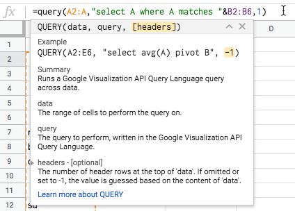
You can press the “X” to remove the whole pane if it’s getting it the way. Or you can minimize/maximize with the arrow in the top right corner.
The best feature of the formula pane is the yellow highlighting it adds to show you which section of your function you are in. E.g. in the image above I’m looking at the “[headers]” argument.
There is information about what data the function is expecting and even a link to the full Google documentation for that function.
If you’ve hidden the function pane, or you can’t see it, look for the blue question mark next to the equals sign of your formula. Click that and it will restore the function helper pane.
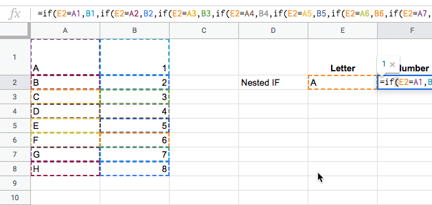
7. Colored Ranges in Google Sheets Formulas
Helpfully Google Sheets highlights ranges in your formulas and in your actual Sheet with matching colors. It applies different colors to each unique range in your formula.
8. F2 To Highlight Specific Ranges In Your Google Sheets Formulas
As mentioned in Step 2, you press the F2 key to enter the formula view of a cell with a formula in.
However, it has another useful property. If you position your cursor over a range of data in your formula and then press the F2 key, it will highlight that range of data for you:
9. Function Name Drop-Down
A great way to discover new functions is to simply type a single letter after an equals sign, and then browse what comes up:
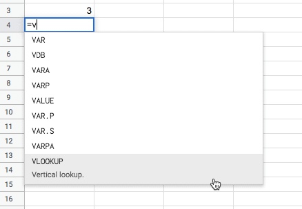
Scroll up and down the list with the Up and Down arrows, and then click on the function you want.
10. Tab To Auto-Complete Function Name
When you’re using the function drop-down list in the tip above, press the tab key to auto-complete the function name (based on whatever function is highlighted).
11. Adjust The Formula Bar Width
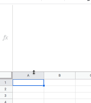
An easy one this! Grab the base of the formula bar until you see the cursor change into a little double-ended arrow. Then click and drag down to make the formula bar as wide as you want.
12. Quick Aggregation Toolbar
Highlight a range of data in your Sheet and check out the quick aggregation tool in the bottom toolbar of your Sheet (bottom right corner).
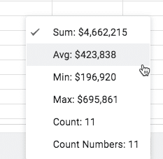
Quickly find out the aggregate measures COUNT, COUNT NUMBERS, SUM, AVERAGE, MIN and MAX, without needing to create functions.
13. Quick Fill Down
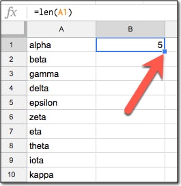
To copy the formula quickly down the column, double-click the blue mark in the corner of the highlighted cell, shown by the red arrow. This will copy the cell contents and format down as far as the contiguous range in preceding column (column A in this case).
An alternative way to quickly fill in a column is to highlight the range you want to fill, e.g.:
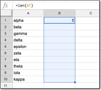
Then press Ctrl + D (PC and Chromebook) or Cmd + D (Mac) to copy the contents and format down the whole range, like so:
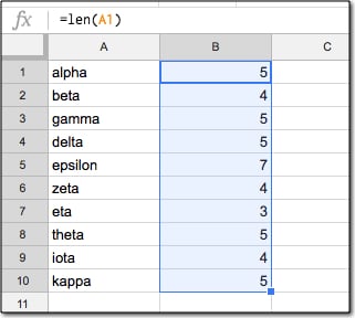
You can also do this with Ctrl + Enter (PC and Chromebook) or Cmd + Enter (Mac), which will fill down the column.
14. Know How To Create An ArrayFormula
Array Formulas in Google Sheets are powerful extensions to regular formulas, allowing you to work with ranges of data rather than individual pieces of data.
Per the official definition, array formulas enable the display of values returned into multiple rows and/or columns and the use of non-array functions with arrays.
In a nutshell: whereas a normal formula outputs a single value, array formulas output a range of cells!
We need to tell Google Sheets we want a formula to be an Array Formula. We do this in two ways:
- Hit Ctrl + Shift + Enter (PC/Chromebook) or Cmd + Shift + Enter (on a Mac) and Google Sheets will add the ArrayFormula wrapper
- Alternatively, type in the word ArrayFormula and add brackets to wrap your formula
15. Array Literals With Curly Brackets
Have you ever used the curly brackets, or ARRAY LITERALS to use the correct nomenclature, in your formulas?
An array is a table of data. They can be used in the same way that a range of rows and columns can be used in your formulas. You construct them with curly brackets:
{ }Commas separate the data into columns on the same row.
Semi-colons create a new row in your array.
(Please note, if you’re based in Europe, the syntax is a little different. Find out more here.)
This formula, entered into cell A1, will create a 2 by 2 array that puts data in the range A1 to B2:
= { 1 , 2 ; 3 , 4 }The array component (in this example { 1 , 2 ; 3 , 4 } ) can be used as an input to other formulas.
One nice application of array literals is to create default values for cells in your Google Sheets.
Read more about arrays in Google Sheets (a.k.a. array literals).
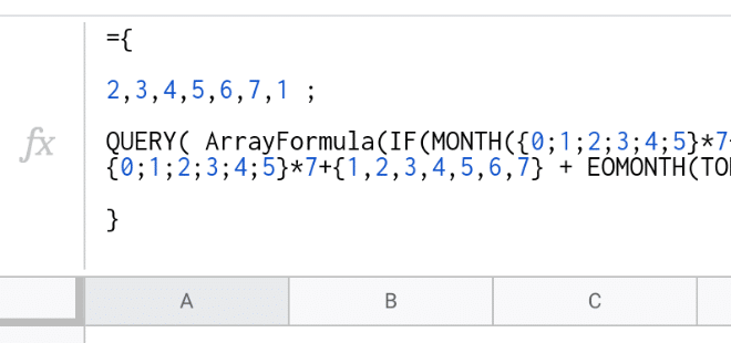
16. Multi-line Google Sheets Formulas
Press Ctrl + Enter inside the formula editor bar to add new lines to your formulas, to make them more readable. Note, you’ll probably want to widen the formula bar first, per tip 11.
17. Comments In Google Spreadsheet Formulas
Add comments to your formulas, using the N function.
N returns the argument provided as a number. If the argument is text, inside quotation marks, the N function returns 0.
So we can use it to add a comment like this:
=SUM(A1:A100) + N("Sums the first 100 rows of column A")which is effectively the same as:
=SUM(A1:A100) + 0which is just:
=SUM(A1:A100)This tip is pretty esoteric, but it’s helpful for any really long Google spreadsheet formulas!
18. Use The Onion Approach For Complex Formulas
Complex formulas are like onions on two counts: i) they have layers that you can peel back, and ii) they often make you cry 😭
Use The Onion Method To Approach Complex Formulas
If you’re building complex formulas, then I advocate a one-action-per-step approach. What I mean by this is build your formula in a series of steps, and only make one change with each step. So if you start with function A(range) in a cell, then copy it to a new cell before you nest it with B(A(range)), etc.
This lets you progress in a step-by-step manner and see exactly where your formula breaks down.
Similarly, if you’re trying to understand complex formulas, peel the layers back until you reach the core (which is hopefully a position you understand). Then, build it back up in steps to get back to the full formula.
For more detail about this approach, including examples and worksheets for each case, have a read of this post:
Use The Onion Method To Approach Complex Formulas
This is an updated version of an article that was previously published. We update our tutorials to ensure they’re useful for our readers.
I’ve been using sheets for years and just learned a number of new shortcuts and answered a couple of questions ive had over time. What a great resource, thank you!
You’re welcome! 🙂
Hello Ben,
I am Google Sheets Trainer, and I’ve found the tip about how to instantly locate the range within the spreadsheet with F2 so useful!
So useful to edit complex formula in big dashboards!
Thank you for sharing your skills!
PS: by the way, I’ve subscribed to your newsletter, and there was a formula challenge on Feb, the 25th (but I have not received the solution if I’m not mistaken). It was:
** FORMULA CHALLENGE – NEW!! **
Start with a straightforward IMAGE function in cell A1
Your Challenge:
Modify the formula in cell A1 only to repeat the image across multiple columns (say 5 as in this example).
Rules: You’re only allowed to use a single formula in cell A1.
Hi Florent,
That’s great to hear 😉
RE: the formula challenge, you can see the solution to that challenge here: https://www.benlcollins.com/spreadsheets/formula-challenge-1-repeating-images-with-array-formulas/
Cheers,
Ben
Great!
Thank you Ben.
Flow.
GREAT……!
Love it! #13 alone is going to save me so much time.
Thank you
You save me so much time.
How can make default value for drop down list?
for example return 0 if it is empty.
Ben ,
Trying to align my formulas in a list or a new line for each query, each time i do this using alt and enter it drops a line. This is what I want but when i click off the formula bar onto a cell it goes back. How do you stop this from happening?
I think the only reliable way to do this is to copy your formula into a text editor, add the spacing you want to have, and then copy it back into your formula bar.
Hope this helps!
Hi
Can you select multiple sheet in a spreadheet, and make same changes over multiple sheets?
Very Nice Sir, It’s really very helpful to boost productivity on Google Sheet during working on Functions.
Great article. Anyone know if its possible to stop google sheets auto-correcting a formula. If I miss a bracket or a comma, I want to make the correction myself to make sure it’s right, but google sheets often just adds a bracket at the end, or takes its guess. Can I toggle that behaviour off?
Also, I want to record some macros to be able to make customised shortcuts that work on all my google sheets. Is that possible, or are macros always just applied to one spreadsheet?
Thanks!
I need absolute references to actually be absolute.
I have a tracker for tracking active data. This is then used for other sheets for filtering and sorting certain entries. When I delete rows that have been completed, and thus need to be removed from the trackers ‘data page’, my formula ranges on other sheets begin to shrink by the number of deleted rows, despite being labeled as absolute, forcing me to go back, and reset the range to the original value. Is there a solution for this in google sheets, a way to get absolutely absolute range references?
Hey JE,
Have you tried leaving the range references open-ended in your formulas, where you don’t specify a end row boundary, e.g. $A$2:$A or $D$2:$D? Hope this helps!
Ben
Hi.
How can I insert what is written in a cell inside a formula of other cell?
For instance:
=HIPERLINK(“https://www.meusdividendos.com/empresa/GOOGL”;”GOOGL”)
an in another cel is writen AAPL
Thanks in advance.
In place of ”GOOGL” in formula direct select the cell (to whome data you want to insert in formula).
Hi
I need a little help
How can change this format
5-7-2001 to 5-7-1
Thanks you
Go to
Format-Number-Custom Date & Time
than create Your format as u want.
Awesome! Thank you for this great info
Hi. How can I put math problems, say down the left side of my sheet, and as students put answers into the second row, if the answer is correct a part of an image shows up – like a huge emoji. But I need to make sure that students aren’t able to edit the document- they only have access to input an answer or change their answer if it’s incorrect. I know it’s possible because I have bought something like this from Teachers Pay Teachers. But I’m going broke, I need to be able to make my own digital worksheets that give the students instant feedback. Thank you so much!
You have to protect whole sheet and give access only Current cell or column to student.
How can I use the F4 short for absolute reference on Macbook Pro with Smartkeyboard?
fn + f4
Really useful article! I’m still trying to find basic info on what “!” and “&” mean in a formula; is there a list somewhere on your site?
I am adding up values in multiple cells and want to add a qualifier that if a certain cell has a “Y” answer, then the end result is 0. If that same certain cell has a “N” answer, the end result will be whatever the sum is of the different cells. This is what I have now – =(D2+F2+I2+K2)+(L2*0.1)-J2
Thanks!
Is there a way to add additional functions into the Quick Aggregation Toolbar in the same way you are able to do so in excel?
Hi Ben,
Unfortunately there’s no way to customize the Quick Aggregation Toolbar at the moment.
Cheers,
Ben
I have 30+ monthly spread sheets. I want the newest spread sheet to show up at the beginning of the list, not oldest sheets at the front of the line.
How do I make this change.
Thank you!
Hi Ben
Not sure how to explain what I am trying to do but here goes
I have a list of clients in google sheets, name address phone etc.let’s call this (sheet 1) in the first column of sheet 1 I would like to use this to type in the sales persons name allocated to this client, and when I do this I would like all the information in the row to be copied onto the sheet (say sheet 2) that is named the same name of the sales person I wish to allocate to the client, the row would ideally stay on sheet one as a master and then the sales member could just look at there sheet. I hope this makes sense and I hope you can help me do this.
Need syntax for multiple IF formulas within one cell that will produce a result based on a criteria in another cell.
To better understand what I am trying to do… For a credit card merchant fee, I have a number of different costs that depend on how a card transaction is performed. Each transaction will have only 1 result. I am thinking I can create a separate cell to designate the formula to use such as IF A,B,C is here use this formula. Any suggestions?
Great resource. I have a weird problem that I hope somebody can help with.
I have this formula to generate a complete formula
B28 =QUERY(‘Incident Detail Report’!A:AW,
B29 “SELECT AW,W,Q,AD,AB,M
B30 WHERE AD CONTAINS ‘Hand(s)’
B31
B32 “)
The above results in a formula
=QUERY(‘Incident Detail Report’!A:AW,”SELECT AW,W,Q,AD,AB,M WHERE AD CONTAINS ‘Hand(s)'”)
My issue is that the query won’t execute unless I copy / paste special value to another cell, and then F2 that cell add a space at the end and them press enter.
The query works perfectly but I want it to execute directly from the formula that creates it. I hope this makes sense.
Hi Ben, for #8, I’m trying to find similar functionality on a Mac. On a PC using F2 seems to act as a “trace precedents” even for complex formulas with references on other sheets. I’ve tried CTRL, Option, CMD + F2 but can’t seem to get it to work–any ideas? Thanks!
Hey Justin, it should work for you on a Mac. You have to position your cursor on the actual range in the formula and then it will take you there.
Hope that helps!
Ben
Hi,
I was wondering why I get a wrong answer on a function on google sheets. For example, I type the following function on an empty cell: =countif(A:A, “<5"), and it returns '0' when it should have returned a number other than 0.
Thanks,
Same formula through different output value
I have a payroll spreadsheet i’m trying to get the same formula my online payroll system has. I’m always a couple of pennys or more off. Mine has =round What do i use instead of round cause the online payroll is not rounding the amount off.
I have a google sheet. It has 2 columns. One for clients I have not reached out to and one for clients that I have reached out too.
I have a lot of clients and receive lists of clients daily to add and some may be duplicates and I want to make sure that I do not reach out to them twice. Is there a way that when I add the additional clients list to the Column for clients I need to reach out too and they are duplicates that it will automatically remove those clients or possible put them in another column for clients I already reached out too? Is there a formula ?
In Excel, if I want to extend the range of cells/data in formula – I double click on the formula cell & then as you can see attached, click on the blue squares in the corners of the selected cells to drag/resize to the area I want extra cells selected etc.
BUT when I do this in Google Sheets, that is, double click on the formula, all that appears is an orange box showing the cells being used in the formula – but I cannot resize it to select more cells?
How do I do this? I don’t want to have to redo the whole formula every time I need to add extra cells or get rid of them from the formula etc?
Thank you!!
I’m working with a number of Google Sheets that have edit/format, download, print, and copy functions disabled. However I can highlight/copy the cell value in the Function Field (Fx) on the Formula Bar.
Is there a hotkey/shortcut moving from a selected cell directly into the Fx field so I can copy that value? Without the shortcut, I’m having to select a cell then mouse-click into Fx field and then double-click to select all the Fx or cell value…
For Sheets that do not have the functions disabled, F2 allows editing a selected cell without moving into the Fx field to give immediate access to edit a portion/typo inside the cell without having to clear the contents when you start typing the entire cell value from scratch. But when the edit/copy functions are disabled, F2 is also disabled. So I need to copy the contents from the Fx field in the Formula Bar.
These formulas are simple and quite easy to remember. Thanks
Ben, trying to figure out how a clients sheet is creating links to other sheets using a double click on the cell without having a typical hyperlink. Its first I have seen. As noted, it will not show the hyperlink modal over the cell to let you confirm the destination.
I use google sheets to track stock $’s. column B
I then have a column with say 85% of the price. column C
I want to retain the lowest column C value.
The problem is as column B changes, so does column C
Is there a way to retain the lowest column C value?