Did you know that formulas are written differently depending on where in the world you’re located? For example, the syntax in the US is different to that in Italy.
This post explores the syntax differences that occur based on your Google Sheets location, i.e. the location you’re working in, assuming your Google settings match (which they would by default).
If you’ve ever copied a template but been unable to get it working, or simply not understood a formula, then it’s possible you’ve run into this syntax issue due to Google Sheets location.
This handy guide will show you the differences and hopefully help you translate seamlessly when sharing Sheets in different locations.
For the most of the world, aside from Europe, you write decimals with a decimal point notation (for example $2.50) and your formulas will use commas to separate the different parts.
I’m currently based in the US, my Google account is set to a US location, so all the articles and template downloads on this site use this notation. (Incidentally, I’m from the UK originally, but since they use the same decimal notation there, formulas in my Google Sheets are the same regardless.)
For countries using decimal comma separators (for example €2,50), which is most of the European countries and a select few others, the syntax for formulas is slightly different, as explained below.
So, ask yourself now where you’re based and how you write your decimal numbers, and then see the different sections below for guidance on how your formulas are written.
How to change Google Sheets location
Before getting to the nitty-gritty of formula syntax, let’s first see where we set the location.
You can specify your Google Sheets location under the File menu:
File > Spreadsheet settings...
which brings up settings pane, where you can specify the Google Sheets location:
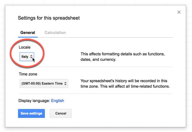
It’s done on a per-Sheet basis, so you can have different locations set for different projects if you require.
Syntax Rules
Locations using decimal points
For locations using periods (or points or dots or whatever you call them) to denote decimal separators (most non-European countries including US, UK, Australia), the syntax will follow this structure:
- Decimals will be denoted by a decimal point (a period)
- Arguments in formulas separated by a comma
- Horizontal data in curly-brace arrays separated by a comma
Locations using decimal commas
For locations using commas to denote decimal separators (most European countries), the syntax will follow this structure:
- Decimals will be denoted by a comma
- Arguments in formulas separated by a semi-colon
- Horizontal data in curly-brace arrays separated by a back-slash
Of course, the best way to understand these rules is to see them in action, so without further ado, here you go!
Formula examples showing change with Google Sheets location
The following formulas, based on the FILTER function, show the different syntaxes side-by-side. Any components that change are highlighted in red.
Basic FILTER example
A) Decimal point notation (e.g. US):
=FILTER( A1:B10 , A1:A10 = "apple" )B) Decimal comma notation (e.g. Italy):
=FILTER( A1:B10 ; A1:A10 = "apple" )In this example, the comma is changed to a semi-colon.
Date Formula example
This formula example shows how to extract the first and last dates of the current month.
A) Decimal point notation (e.g. US):
=EOMONTH( TODAY() , - 1 ) + 1=EOMONTH( TODAY() , 0 )B) Decimal comma notation (e.g. Italy):
=EOMONTH( TODAY() ; - 1 ) + 1=EOMONTH( TODAY() ; 0 )In this example, the comma is changed to a semi-colon.
VLOOKUP Formula example
A) Decimal point notation (e.g. US):
=VLOOKUP( F1 , A1:C10 , 2 , FALSE )B) Decimal comma notation (e.g. Italy):
=VLOOKUP( F1 ; A1:C10 ; 2 ; FALSE )Again, the comma is changed to a semi-colon.
Curly-brace Array Formula example
A) Decimal point notation (e.g. US) use a comma within the curly-braces array notation to create arrays in Google Sheets in the same row, like this:
= { 1 , 2 }and a semi-colon to create data arrays in the same column, like so:
= { 1 ; 2 }which give the outputs, respectively:
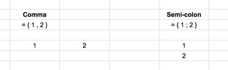
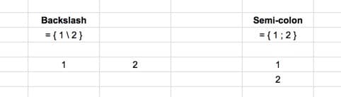
B) Decimal comma notation (e.g. Italy) use a back slash within the curly-braces array notation to create arrays of data in the same row, like this:
= { 1 \ 2 }The vertical orientation does not change, and still uses the semi-colon to create data arrays in the same column, like so:
= { 1 ; 2 }which give the outputs, respectively:
So let’s see an application of this array syntax rule with the SPARKLINE formula.
SPARKLINE example
A) Decimal point notation (e.g. US):
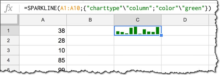
=SPARKLINE( A1:A10 , { "charttype","column" ; "color","green" } )B) Decimal comma notation (e.g. Italy):
=SPARKLINE( A1:A10 ; { "charttype"\"column" ; "color"\"green" } )There are two things happening here:
i) Inside of the curly braces { ... } we apply the array syntax rules, so the comma changes to a back-slash, but the semi-colons do not need to change.
{ "charttype","column" ; "color","green" }changes to:
{ "charttype"\"column" ; "color"\"green" }ii) Outside of the curly braces, in the main part of the formula, where the arguments are separated by a comma in the decimal point notation, they’re separated by a semi-colon in the decimal comma notation. (I realize that sentence may be somewhat confusing! What’s happening is this:
=SPARKLINE( A1:A10 , { ... } )changes to:
=SPARKLINE( A1:A10 ; { ... } )And that’s as complex as it gets.
If you can remember your rules and check whether you’re operating inside of a curly brace array or not, then you should be able to convert formulas between different locations.
Default currency, date, and number formatting
Since we’re on the location topic, it’s worth spending a couple of minutes seeing what else changes.
The default currency of the Sheet will match the currency that is used by the location set for the Sheet. So if you’re Sheet is set to US, you’ll get the Dollar sign ($) when you use the currency formatter. In Europe, you’ll get the Euro sign (€), whilst in the UK, you’ll get the Pound sign (£).
Similarly the default date format will match the location, notably that US dates will appear with the Month preceding the Day, so MM/DD/YYYY, whereas everywhere else will go with the Day first, so DD/MM/YYYY. (Incidentally, this took me a long time to get used to when I first arrived in the States!)
And finally, number formatting follows the decimal point or decimal comma style that we’ve discussed all the way through this post, so $0.99 versus €0,99
Further reading
Google documentation on changing a spreadsheet’s location
Google documentation on using Arrays in Sheets
The full list of decimal comma countries is here.
Further reading on FILTER function
Further reading on Array Formulas
If you’re into formulas, be sure to check out my free Google Sheets course: Advanced Formulas 30 Day Challenge
Thanks, I was scratching my head, wondering what denotation should be used, as I specifically remembered using commas, while also knowing that commas shouldn’t be right. Though I have to admit that I have no recollection of ever using back slash in arrays, but maybe I’ve only done vertical arrays.
This is really helpful, and I’d like to ask a follow-up question. How do I use curly brackets to arrange data as follows?
I have data in Qns!A2:D31 which I need to move around a bit.
I want a pair of columns 60 rows long where the top half shows A2:B31 across the two columns, and the bottom half shows (and this is the hard bit) D2:D31 in the left-hand column and C2:C31 in the right-hand column.
I tried to do this with
={Qns!A2:B31;query(Qns!C2:D31,”SELECT col2,col1″)}
but I get a #VALUE! error.
I’m using periods as decimal points, not commas.
Thanks a lot for this extremely useful, well-written, and well-documented article with lots of helpful clarifying examples. Kudos!
However I suggest you check your facts on the use of decimal comma vs. period in the world. The number of countries using the decimal comma far exceeds that using the period, even if you ignore Europe entirely. In number of users however the decimal period dominates due to China and India. Basically the formula goes “China and former British colonies use the period, the rest the comma”.
Funny you include the UK in non-European countries 😉
(just below the syntax rules)
There’s a wikipedia article on the topic (https://en.wikipedia.org/wiki/Decimal_separator) where you can see that Ireland and some cantons of Switzerland use the dot too.
Thank you so much!
I was going nuts trying to get my two-dimensional array to work on a Nordic locale. I really wish Google would keep a decent list of updated syntax notation for all locales in their documentation.
This is brilliant! So happy I remembered that I’d just recently seen this mentioned somewhere, so when I searched for it I found it right away. Anyway, I have a follow-up question which is also based on another trick I’m sure I picked up from you, Ben.
I’m using the “is this the first row trick” with ARRAYFORMULA to create a header, and then display data from row two. But combining that with this idea, I need to add two separate headers, and currently I can only add one. Check this out.
=ARRAYFORMULA(IF(ROW(C:C)=1;”Licence”;IFERROR(ARRAYFORMULA(VLOOKUP(A:A;Licenses!$A:$E;{4\5};FALSE)))))
As you can see this puts “Licence” into C1, and the VLOOKUP results into C2:D, but I also need to put “License name” into D1, and I don’t know how to do that.
Please advise.
Hi Ben, I need to know how can I add a Cell reference instead of the function mentioned below.
=query(A6:C,”select C, count(C) where B > date ‘2000-01-01’ group by C”,1)
Regards,
Parag Shah
Hello – i’m struggling with the following formula – i live in France, so have tried changing the syntax according to your rules, but am in a muddle! IFS($C9=””;””;$G9/$C9;SPARKLINE($V9;{“charttype”\”bar”;”max”\100%;”color1″\”#5e9cf7″;IFS(V9=34%;V9=67%;”green”;”empty”\”zero”})))