The Google Sheets Filter function is a powerful function we can use to filter our data. The Google Sheets Filter function will take your dataset and return (i.e. show you) only the rows of data that meet the criteria you specify (e.g. just rows corresponding to Customer A).
Suppose we want to retrieve all values above a certain threshold? Or values that were greater than average? Or all even, or odd, values?
The Google Sheets Filter function can easily do all of these, and more, with a single formula.
This video is lesson 13 of 30 from my free Google Sheets course: Advanced Formulas 30 Day Challenge.
What is the Filter function?
In this example, we have a range of values in column A and we want to extract specific values from that range, for example the numbers that are greater than average, or only the even numbers.
The filter formula will return only the values that satisfy the conditions we set. It takes two arguments, firstly the full range of values we want to filter and secondly the conditions we’re going to apply. The syntax is:
=FILTER("range of values", "condition 1", ["condition 2", ...])where Condition 2 onwards are all optional i.e. the Filter function only requires 1 condition to test but can accept more.
How do I use the Filter function in Google Sheets?
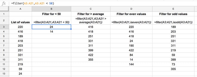
For example in the image above, here are the conditions and corresponding formulas:
| Conditions | Formula |
| Filter for < 50 |
=filter(A3:A21,A3:A21<50)
|
| Filter for > average |
=filter(A3:A21,A3:A21>AVERAGE(A3:A21))
|
| Filter for even values |
=filter(A3:A21,iseven(A3:A21))
|
| Filter for odd values |
=filter(A3:A21,isodd(A3:A21))
|
The results are as follows:
(Note: not all the values are shown in column A.)
Click here to get your own copy >>
Can I test multiple conditions inside a Google Sheets FILTER function?
Absolutely!
For example, using the basic data above, we could display all the 200-values (i.e. values between 200 and 300) with this formula:
=FILTER(A3:A21, A3:A21>200, A3:A21<300)Can I test multiple columns in a Filter function?
Yes, simply add them as additional criteria to test. For example in the following image there are two columns of exam scores. The Filter function used returns all the rows where the score is over 50 in both columns:
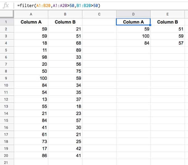
The formula is:
=FILTER(A1:B20,A1:A20 > 50,B1:B20 > 50)Note, using the Filter function with multiple columns like this demonstrates how to use AND logic with the Filter function. Show me all the data where criteria 1 AND criteria 2 (AND criteria 3...) are true.
For OR logic, have a read of this post: Advanced Filter Examples in Google Sheets
Can I reference a criteria cell with the Filter function in Google Sheets?
Instead of hard-coding a value in the criteria, you can simply reference another cell which contains the test criteria. That way you can easily change the test criteria or use other parts of your spreadsheet analysis to drive the Filter function.
For example, in this image the Filter function looks to cell E1 for the test criteria, in this case 70, and returns all the values that exceed that score, i.e. everything over 70.
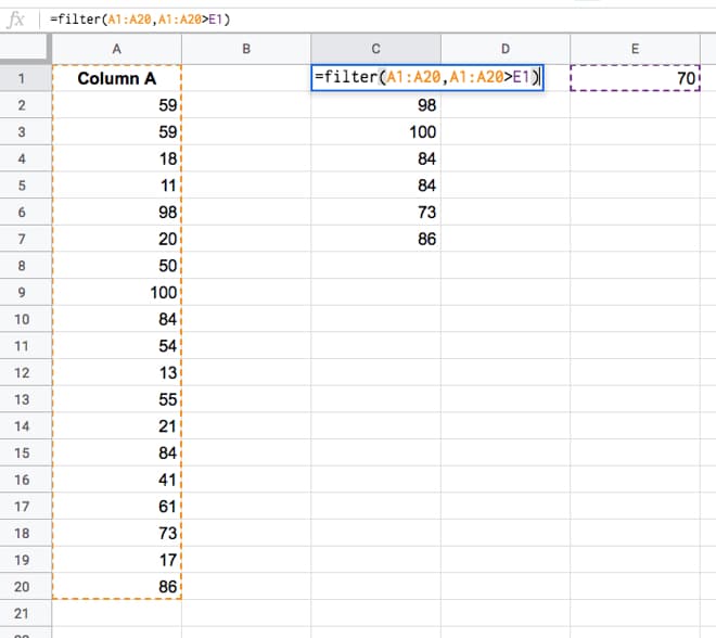
The formula in this example is:
=FILTER(A1:A20,A1:A20 > E1)Can I do a filter of a filter?
Yes, you can!
Use the output of your first filter as the range argument of your second filter, like this:
=FILTER( FILTER( range, conditions ), conditions )Resources
Advanced Filter Examples in Google Sheets
Google documentation for the FILTER function.
Related Articles
 Advanced Filter Examples in Google Sheets
How to use an advanced filter with an OR condition in Google Sheets. Knowing the trick will save you hours, so you can filter multiple conditions easily.
 Google Sheets Query function: The Most Powerful Function in Google Sheets
Learn how to use the super-powerful Google Sheets Query function to bring the power of SQL to your data, with this comprehensive tutorial and available template.
Good stuff. Thanks for this. Saved me a lot of time.
Do you know if there is a way to return the values horizontally instead of vertically? For example if there were 4 results and the formula was in cell B2 then the results would be in B2, B3, B4, B5. Is there a way to instead have the results return in cells B2, C2, D2, E2?
Thanks!
Hey Burton,
Just wrap your formula with this one:
TRANSPOSE()and that will flip from vertical to horizontal or vice versa.e.g.
=ArrayFormula(transpose(filter(A2:A20,iseven(A2:A20))))Hope that helps.
Cheers,
Ben
Hi there, what would be the best way to do this in google sheets…make a list of students who have a score of 0 for at least one assignment. It has over 50 students and 15 tests listed. Showing you a super short sample below. Thanks in advance for your help.
student 1 0 1 0 5
student 2 5 6 3 2
student 3 2 0 1 8
fastest way to do that if it’s just a 1 off query would be to add a column at the right of the test scores to countif any cells in the current row = zero. Then filter the whole column to remove zeros. You are left with all rows which have at least 1 score = zero.
Hi Ben,
I am looking to filter any of 3 columns containing the same data. Meaning, I have machine operators that may appear in any of three columns and I want to see any place where they show up. If I filter by their name in one column the rows in which they appear in other columns disappear and the option of choosing them in those filters also disappears. Any ideas how to solve this?
Thanks
Brian
You are simply Great Ben.
How do I make a totals row that counts the numbers for only the data that is being filtered?
So I have a list for a committee meeting that I just want to show a total for the attendance, Ideally Id like to filter by employee and month. Currently the sum function counts every single entry and I would like it to automatically sum as i filter the data.
You can use TRANSPOSE to flip any array from horizontal to vertical (or vice versa), including arrays generated by other functions.
I really like this function. Query is other that is really interesant forme because you can do pivot tables. Both are awesome! some days ago I test an addon for google that allow you import filtered tabs (importsheet.com). Its great.
Rewards!
Hi,
How do I create an exact match using filter function?
For example: I would like to have food and Food to match exactly.
food 10
Food 12
Hey Christina,
If you want to match a condition exactly, then your formula will be:
=filter(A1:B10,A1:A10="food 10")assuming your range is in A1 to B10, with the search values (the filter values) in column A.
If you wanted to modify this to be “food 10” or “Food 12”, then your formula becomes:
=filter(A1:B10,(A1:A10="food 10")+(A1:A10="Food 12"))Hope that helps!
Ben
Hey Ben!
Thank by your post. Now I am using “filter” function in one sheet and everything is working well!!!! 😉
Many thanks!!!
I needed to do this and used regexmatch
Hi Ben,
Can I filter a column, say A:A, by conditions in another column, say B1:B8? Obviously Column B has less cells than Column A.
Thanks,
Kelvin
Hi Ben,
Would it be possible to use the filter function to create a list of unique values using data from multiple sheets that meet a criteria found in another column on those sheets? For example, I want to create a list of all the times of day when only a specific kind of workshop was given and this data is spread across multiple sheets.
Thanks!
Very good
Hi Ben,
Would filters be appropriate to return only the last row for a set of observations for several samples?
sample, value, date
1 4.5 2017-02-14
1 4.3 2017-02-17
1 4.5 2017-02-18
2 4.2 2017-02-14
2 4.3 2017-02-17
2 4.6 2017-02-18
3 2.3 2017-02-14
3 2.1 2017-02-17
…
I really just want to be able to see the last observation row for each sample from ColA. Sometimes, the value happens to be the largest for that sample, but not always. Also, some dates might not have an observation for a particular sample, so dates don’t seem to be a reliable thing to use either.
Thanks!
Romeo
Hey Romeo,
Yes, you can use the filter function to achieve this. Taking your dataset and assuming it’s in cells A1:C9 (although can be as many rows as you want) then you can use this formula to retrieve only the last row of data (specifically the last row with a value in column A. Also this formula assumes no gaps in the values in column A):
=filter(A2:C,(A2:A<>"")*(A3:A=""))Just make sure not to put this formula in columns A, B or C since they have your data in. Hope that helps.
Cheers,
Ben
Thanks for the quick reply!
This doesn’t work for me (but it DOES perfectly give me the last row). I’m not sure if I was clear:
I want the last row for EACH sample number, so my desired result from the data above would be:
sample, value, date
1 4.5 2017-02-18
2 4.6 2017-02-18
3 2.1 2017-02-17
Does that make it clearer?
Thanks!
Ah, I see what you mean now. Thankfully an easy fix 🙂
Try modifying the formula to this:
=filter(A2:C,(A2:A<>"")*(A2:A<>A3:A))Yep! That’s awesome!
I have been struggling with this for several months…it’s a hard question to even ask, it seems.
Thanks a million,
Romeo
Great! Happy to help.
Cheers, Ben
I need help I need to filter numbers
{2, 34, 56, 59, 70}. For example I need to know the sum of second and first numbers sum of the third and second number the sum fourth and third number and the sum fifth and fourth number .The sum in between the numbers and added and subtracted I need a easy way to do this please added in one subtracted beside it i don’t want to take for ever doing this
Hi Ben!
Is there a way for the filter formula to return data from two different tabs on the same sheet? I am collecting communication data using a google form and my texting platform’s API, so unfortunately I cannot consolidate tabs. Still, I want to be able to see individual communication logs for each person. Does that make sense?
Thank you!
Hey Erin,
Missed this comment when you originally posted, so this is a bit late 😉
You’d first want to combine your data ranges from the different tabs into one data range, and then use the filter function on this combined data range.
You can combine your data ranges with curly brackets, e.g. this formula would stack data from Sheet1 columns A & B, with Sheet 2 columns A & B:
=sort({'Sheet1'!A1:B;'Sheet2'!A1:B},1,true)You’d put this formula in a new tab, then put the filter function next to it, pointing at this data range.
Cheers,
Ben
This is great! Thank you! There is an issue though. I have 2 sheets gathering data from forms. I can combine the data in one sheet but i cannot filter if some of the cells are empty (i get an error). Is there a workaround?
Does this Filter feature work for multiple columns of data? I’ve been using an importrange function to import a table of data from one tab to another, turning it into a Filtered Table, and then manually filtering by specific text.
The issue is I have to manually set the filter condition and if I update the original data table then I have to revisit all subsequent tabs to update.
Hey Jasmine,
I think I get what you’re issue is… and yes, the filter function does work for multiple columns, you just add them after a comma in the formula. Here’s the syntax:
FILTER(range, condition1, condition2, ...)And here’s an example with some filter applied to column A and D:
=FILTER(A2:B26, A2:A26 > 5, D2:D26 < 10)Hope that helps!
Ben
Could this be used to calculate a percentage of task done. So if Column C is blank then go to Column 0 and if – count as zero if date entered count as 1 to calculate what percentage of task in Column 0 is completed?
Not sure I understand your question here… sounds like you might want to do a COUNTIF (or SUMIF if you have 0’s and 1’s) based on your condition and then divide by the total of items to get a percentage completed.
Hi Ben
If I’ve got my main data on Tab A, and I have applied a filter to see what I need to on Tab B, can I get Tab B to update automatically whenever new rows get added to Tab A (i.e. new rows will appear on Tab B automatically if I have added a row to Tab A that matches the filter)?
Thank you!
Anna
Yes, you can! When you reference Tab A in your filter, make sure you don’t specify a final row in the range, e.g. your range should look like this:
'Tab A'!A1:Dwith no number at the end. That way the range extends all the way to the bottom of your sheet so new data will be included.
Cheers,
Ben
Hi, i have a sheet that contains column with names, column with dates and column with Quality Score. For example on 10/1/2017, I have 5 unique names and each names have multiple rows with survey and quality score ratings. The name John has 5 rows with quality score on all rows, the names michael and charlie both have 5 rows as well but not all rows have quality score, 3 out of 5 rows are blank, the last 2 names are Bob and Eman with 5 rows but all rows show blank on quality score. What I’m trying to do is im trying to pull the names that doesn’t have quality score at all or show blank on all rows for quality score.
Hi Zyre,
You’ll want to do something like this:
=filter(A:C , C:C<>"")where I’m assuming your three columns are A, B and C, and that the quality score column is column C. This formula will return all the non-blank values. You can add other conditions into the filter too.
Cheers,
Ben
How would I filter to only include blank cells in C:C? I want to filter and show those rows where customers did not fill in a certain field.
I can filter to include not blank cells, but not empty cells. Any help would be appreciated.
BTW, love the videos and the articles. Great help for me!
I am trying to filter a sheet that has 55,000 rows. I need to get that to a manageable size as most of those rows are irrelevant to my needs. The filter formula I have in place works fine, but requires me to put finite ranges(A4:A1500, etc.). It works up to 15,000 rows, but anything over that tells me no matches are found. I am changing both the search range, and condition range to the same parameters. Any Ideas???
Hey Adam,
Does it work if you put ranges like A4:A, without specifying a final row? Haven’t heard of this problem before or seen a solution.
Cheers,
Ben
Hi Ben, Great post! Is there a way to filter a column by the color of the text in each cell? Or by the background color of the cell? Or by cells with bold or italicized text? I can do this in Excel but haven’t been able to easily find a way in Sheets.
Thanks! Cammie
Hey Cammie,
Unfortunately not in Sheets. One of the features Excel has that Sheets doesn’t (yet) 🙁
Ben
Hey! Trying to filter for forms that are expiring within 30 days, and currently using the following formula: =FILTER(Students, G:G > (today() – 30)), where Students is a named range containing all the relevant data, and G is a column with expiration dates in it. When I try to apply the filter, I get an error:
Error
FILTER has mismatched range sizes. Expected row count: 156. column count: 1. Actual row count: 1000, column count: 1.
Any tips on how to get around this?
Hi Ben,
Great content as always!
I read all the comments and I can’t find a similar question. I have to filter data from an importhtml and I want to have all the cell with the text beginning with “/market/”. My problem is that I can’t filter using an exact match as there is other text after this (and that is atually the information I need..). What can I do?
Hi Bin,
If I have range containing below values:
A
B
C
D
A
D
C
B
How should be filter function written to give this result:
A
B
C
D
A
B
C
D
Great post
But is it possible to filter some range for two values?
(e.g: filtering a table with specific date range and category of payment)
Yes! You can add more conditions into your filter formula using the same syntax, like so:
FILTER(range, condition1, [condition2, ...])Hi Ben,
Thank you for the tutorial! I have a big google sheet and i want to make a web page were users can manually filter the database . So they will make choices from a menu and the page will give them the filtered google sheet back.
How can I implement the user response into the formulas?
I have a main sheet and I want to create another sheet in the same workbook that pulls information ie. if agent name is John on the main sheet then it will auto populate on the other sheet named John with the specific columns required ie. address, commission %, commission $, etc. Can this be done?
Hi Ben,
Thanks for your site !
I ask myself if it’s possible to make a FILTER of a SORT on more than one sheet in the same GOOGLE SHEET FILE ? I find notging about that and you’re the specialist ! Thank you.
Oh sorry i wanted to say FILTER or SORT. Thanks.
Hi Audry,
Not exactly sure what you mean, but since the filter and sort functions take ranges as inputs, you could potentially combine data ranges with the {} array notation to pass into the filter or sort, e.g.
=sort({'Group A'!A1:B;'Group B'!A1:B},1,true)This will combine my data from Group A sheet with data from the Group B sheet and then sort the combined data. It does require that the data in A and B are the same format and same headings etc.
Cheers,
Ben
In the examples at the top of the article, why do you wrap in ArrayFormula for the last two, but not the first 2?
Good question! The last two need the ArrayFormula construction because of the inner function ISEVEN, which is applied to a whole range. Therefore I need to denote it as an ArrayFormula so it’ll apply to every cell, not just the first.
Actually, scratch that! The last two will work without array formulas. I’ll update the article.
Can i create a filter inside a filter formula? i.e. something like =filter({filter(range,condition)},condition)
Yes, you can do that!
Note: you can also have multiple conditions inside of a single filter function:
=filter(range, conditions 1, conditions 2, etc.)Hi Ben. I really like this function! I’m may have an add-on that can help you to not only filter but also connect your data.
Would like to invite you to test.
http://www.sheetgo.com
Would be awesome have your feedback.
Regards
Mariana
Hi,
I am using Google sheets to filter data based on a selection criteria.
I have multiple instances of this:
INDIRECT(“‘Data Feed (WD8)’!L1:L10000”)=’Sales Manager View’!T7)
So the user can select what they like to see (within a cell like T7) and then the data will automatically filter. The problem I have is I don’t know how to bring back ALL for multiple criteria. The drop-down has a list of business units in this example. I thought what I could do is simply get the user to type into T7. I can do this, it works, but then if I try to do it on multiple fields then it breaks (no matches are found in FILTER evaluation). So I can’t use more than once in this formula?
What am I doing wrong?
Thanks,
Dave
Hi Dave,
You can wrap your filter with an IF statement to deal with the ALL case, like this:
=IF( T7 = "All" , return all the data , FILTER(....) )Ben
Further to above, I tried to put two symbols which haven’t come through on the post but it was meant to read:
I thought what I could do is simply get the user to type {less than more than} into T7. I can do this, it works, but then if I try to do it on multiple fields then it breaks (no matches are found in FILTER evaluation). So I can’t use more than once in this formula?
Hi Ben, great article! Filter is a core function of a lot of sheets I run; can’t live without it!
Found myself helping someone with their Form data filtering for two columns of criteria to count the number of times value X appears. Using some form validation they can pick their different criteria. Easy enough!
However, sometimes they want to see the count for one criteria and any/all for the other. A blank cell in either drop down cell returns the dreaded #N/A.
Is there an way I can tell the filter to match any criteria from the cell? An asterisk style command of sorts?
Scaled down formula:
=COUNTIF(filter(‘Form Responses 1’!J2:J, ‘Form Responses 1’!B2:B=A2, ‘Form Responses 1’!C2:C=B2), “Yes”)
I cobbled together a solution, in case anyone runs into a similar situation, by using IFS to string together my different criteria, ISBLANK for my empty dropdown scenarios, and 2 inverse ISBLANK statements for when both dropdowns are filled. This was the final result:
=IFS((AND(not(ISBLANK($A2)),not(ISBLANK($B2)))),(COUNTIF(filter(‘Form Responses 1′!$J$2:$J,’Form Responses 1′!$B2:$B=$A2,’Form Responses 1’!$C2:$C=$B2),D$1)),
ISBLANK($A2),(COUNTIF(filter(‘Form Responses 1′!$J$2:J,’Form Responses 1’!$C$2:$C=$B2),D$1)),
ISBLANK($B2),(COUNTIF(filter(‘Form Responses 1′!$J$2:J,’Form Responses 1’!$B$2:$B=$A2),D$1)))
Great to hear you got this sorted! 🙂
Hey guys,
I have a master sheet that has 100+ different entries on it, each with a series of criteria to query (Colour, Width, Length, Height, Weight, etc…).
I have a Summary sheet where I’ve created a bunch of drop-downs to indicate which entries you would like to see, depending on the criteria selected, and I have a list per criteria that displays any corresponding entries, based on that ONE criteria.
What I am TRYING to do is have a list that feeds back only the entries that match ALL the selected criteria.
For instance –
I have selected the Colour RED, the Width 10, and the Height 50. Each of the discreet, per-criteria lists returns all the entries that correspond with the query, but what I would really like is a list that tells me all the entries that are RED, have 10 Width AND 50 Height.
Any ideas on how I can get this done in Google Sheets?
I think I’m looking for the same thing as Gord. I have a Database of routes to fly (Tab 1 = Database). Columns = Airline, Flight Number, Departing ICAO, Arriving ICAO, Depart Runway, Arriving Runway, and then some other info that won’t be filtered but will show up with the results of the filtered columns.
I then on another tab have A1:A6 with the different columns from the other sheet titles. And in B1-B3 I have a drop down menu to select the Airline, Departing ICAO code and Arriving ICAO Code. Then once those results show you can type in B4-B6 the flight number, and Runway info you want to show based on what is showing from the filter (no drop down menu).
The problem with the filter I am using now is that when one of the B1-B6 entries are empty, it is not filtering at all. All the B1-B6 criteria have to be filled in for it to work. How do I get it to work if I only put in Criteria fro some of the columns im filtering for but not all of them?
Here is my Formula, basically this: =filter(range, conditions 1, conditions 2, etc.)
=FILTER(‘Database’!A2:J, ‘Database’!A2:A=B1, ‘Database’!C2:C=B2, ‘Database’!D2:D=B3, ‘Database’!B2:B=B4, ‘Database’!E2:E=B5, ‘Database’!F2:F=B6)
Database Tab Set up (Column):
Airline
Flight#
DepartICAO
ArriveICAO
DepartRwy
ArriveRwy
FlightLevel
Route
FlightPlan
FlightAwareLink
Filter Tab Set up:
A1 = Airline, B1 = drop down menu of all the Airline options
A2 = Departing ICAO, B2 = drop down menu of all the ICAO Code Options
A3 = Arrival ICAO, B3 = drop down menu of all the ICAO Code Options
A4 = Flight Number, B4 = manually type in a flight number once above is showing
A5 = Departing Runway, B5 = manually type in a runway# once above is showing
A6 = Arriving Runway, B6 = manually type in a runway# once above is showing
It won’t work if one of the above is empty.
Hi – Simple question…how do I get back to my original view after creating a few different filters?
The filters work great for seeing different important aspects of the data, but now I want to go back to the original layout before I applied these filters.
My filters are doing nothing but sorting by three of the columns to group the data differently.
I’m sure I’m overlooking an incredibly obvious thing here… !
Hi Terry,
You can dropdown all the filters you’ve applied and choose “Select all” again to show everything in that column. If you’ve filtered multiple columns you’ll need to do it for each one. Shame there’s not a global “Select all” option in the filter menu.
Alternatively, it’s sometimes quicker just to remove the filters altogether (from the toolbar above the Sheet), which will show all your data again. Then you can reapply it if you want to start over.
Note, you can also save a particular filter view if you want to return to it. That option is in the Filter menu on the toolbar.
Cheers,
Ben
Ben,
Can I use the FILTER function to remove blank cells from a range?
Currently, I have a 70-cell vertical range in my spreadsheet (B66:B135) but only 11 cells are not blank. (All values in the range are numbers generated from a formula). I’m using =FILTER(B66:B135,B66:B135″”) in cell B139, but the formula isn’t giving me correct results.
What formula can I use to get a concise list of non-blank values? I’d like to do this without any user interaction at all. (Extra credit if I can sort the output to ascending values.)
Thanks,
Henry
Hi Ben,
Love your work – starting the 30 day challenge real soon. 🙂
Quick question, which hopefully has an easy answer, though i can’t think of one at the moment, but filter is coming close.. i hope.
Situation.
Sheet 1 has multipe numbers in different rows and colums, combined with text. It’s a email template sheet where i fill in the article ids that has to come in an email. It then loads the images with =image(vlookup in the productfeed), and titles etc.
Now i would like to extract all those articles id’s (not campaign text) in a different sheet into one column. Is filter the right formula?
Much appreciated!
Best,
Berend
The difficulty I am experiencing is that I use filter (and query sometimes) and when the length of the returned data (i.e. number of rows) is less than the previous instance, the “old” data is left over. Filter does not understand the maximum length of the resulting area in order to clear out old results.
It’s probably not good form to answer your own question, but in case someone had a similar issue a found a way that helps me …
I was filtering a range of rows (8 columns wide). By using a formula of the following style, I could append enough blank rows to always overwrite any “old” data
={filter(……codes …) ; range} adds the extra rows I needed to overwrite the old data. The range has to be the same width as the filter range.
Thank you for this; saved me a lot of time!
I need some further help, however.
I have successfully filtered 1000 rows of data down to around 250. I need to make changes to the formulas of these filtered cells now before moving on but it won’t let me. Each time I change the data, it returns back to the original filtered data. How can I get around this problem?
TIA!
Hello!
Really great function. Do you know if i can use a filter that takes information from another workbook?
Thanks.
Hey Julia,
You can’t use data from a different Google Sheet without first bringing it into your current Sheet, using the IMPORTRANGE function. The FILTER function can only directly access data in your current Google Sheet.
Cheers,
Ben
Hi Ben,
How do you use FILTER function when the cell contains the text that I want. I’m not going to use the exact text, just contains.
I want to filter all the rows that contain the word “task”.
Best,
Cris
Hey Chris,
This is a little tricky to do, but your formula would look something like this:
=FILTER(A1:B10, ArrayFormula(REGEXMATCH(A1:A10,".*task.*")))assuming your data was in range A1:B10, and the column A1:A10 had your text values you’re filtering on. You can obviously change these ranges to match your example.
Cheers,
Ben
Hi Ben, if the search item to be filtered is a number, will the formula be changed?
Hello Ben, I generally find answers here but I’m stuck today.
I try to filter a range with multiple approximate criteria.
I started with 1 criterion, this works well for me
=FILTER(A1:B10, NOT(ISERROR(FIND(“task”,A1:A10)))
This does not work
=FILTER(A1:B10, ArrayFormula(REGEXMATCH(A1:A10,”.*task.*”))) .
I’d like to filter all tasks related to me for example.
=FILTER(A1:B10,
NOT(ISERROR(FIND(“task”,A1:A10)),
NOT(ISERROR(FIND(“jean”,A1:A10))
)
this works.
I want to input in a cell “jean task” or “task jean” and generate automatically the latter function.
Any idea ? 😀
thanks
Jean
Thanks a lot, Ben! This is very helpful.
Hi Ben,
Thanks a lot for the previous help.
I have another favor to ask.
I have 3 sets of columns(each has a different filter). What I’m trying to do is align the columns horizontally.
The number of rows per column varies every time there is an update.
Here is a link to a doc with images(cause it’s hard to explain): https://docs.google.com/document/d/1w3FMYsvAublYqF1vs4B_4iG7Qi0CUTxpCzNlgVfvylM/edit?usp=sharing
I really appreciate the help thanks you in advance.
Kind regards,
Cris
Hey, I have a filter code that returns me several text lines
=FILTER(K1:K;J1:J=1)
And I would like to get the last 2 words of each row. I’d normally achieve that with this code:
=RIGHT(U2;LEN(U2)-LEN(JOIN(” “;ARRAY_CONSTRAIN(SPLIT(U2;” “);1;COUNTA(SPLIT(U2;” “))-2)))-1)
But I wonder if I can implement the last code into the filter function.
Hi Ben,
I have a doubt / looking for a solution in getting one value from a specific row.
Scenario:-
Sheet 1 : – I have column A [integer] and B [different labels] total 52k data in one column].
Sheet 2:- I have columns till H, only the A column has different labels and sheet 1 B column are same.
From Sheet 2 to i gave have to do the following formula
1. Sort the Sheet 1 – got it done manually
2. Filter for one unique value [total 21 unique value]in Sheet1!B – completed
3. Take count and do a the percentile calculation – completed [=ROUND((90*(F2+1))/100)] *F2 is the count value
4.Take the value from the above and go to sheet 1 and column A and copy the value in the specific row – ? in this one can you help
got the answer myself
=INDEX(filter(Data!$B$2:$C$52257, Data!$C$2:$C$52257=”<Text Name"),$J2 , 1 )
Hey Ben,
How do you use the FILTER function when I want return all the different types of texts in a column.
For example, column C:C contains Gear, Equipment, Products and I want all three to show not just one
I used this filter to return only one condition
=filter({‘Form Responses 1′!A:A,’Form Responses 1′!E:E,’Form Responses 1′!D:D,’Form Responses 1′!F:M},’Form Responses 1’!C:C = “Gear”)
Hope I exampled this
-P
Hi Paulita,
You can try using ‘+’.
Like this:
=filter({‘Form Responses 1′!A:A,’Form Responses 1′!E:E,’Form Responses 1′!D:D,’Form Responses 1′!F:M},{’Form Responses 1’!C:C = “Gear”}+{’Form Responses 1’!C:C = “Equipment”}+{’Form Responses 1’!C:C = “Products”})
Let me know if it doesn’t work.
Kind regards,
Cris
Hi,
Thanks for the info on the Filter function. I have a multi-user sheet with a master list. Other users can update data in the list, but I as administrator would like to limit (filter) the records they can see/edit.
I have a cell which defines the filter which i will update from another sheet. When the user opens the sheet I would like it to present them with the filtered list, and allow them to edit fields (they would not edit any fields used for filtering).
If I use the FILTER function, it copies the filtered data to another place, but I can’t see how edited data would feed back to the master list. If I use the FILTER dropdown command, I don’t know how to have the filter update based on an external source (someone physically has to click on the dropdown to change the filter).
Is there a solution here? Many thanks!
I too have this issue…did you figure anything out?
I have a filter that I’m using that works perfectly for exact matches and have been playing around trying to get it to work with partial matches using regexmatch and an not having any luck. Here’s what I’m using for my filter for the exact match when the value for what I am searching is entered into cell A1.
=filter(‘VIEW ALL Partner Assignments’!B:B,’VIEW ALL Partner Assignments’!B:B=A1)
Hi Maaureen,
Please try this:
=filter(‘VIEW ALL Partner Assignments’!B:B,(ArrayFormula(REGEXMATCH(’VIEW ALL Partner Assignments’!B:B,A1)))
Kind regards,
Cris
Hi Ben,
First, I would like to thank you for these awesome tutorials and I learned alot!. However, during my actual creation of some filter commands I encountered a problem with copying values inside a merge cells from a multiple rows. I dont know if I say it correctly but you can check this google sheet (from you) and I just added 2 test sheets named;
1. MainSheet – Which have the details I need for the filter
2. FilterSheet – Which the sheet I used to run the filter formulas.
I was able to achived a part of my mission here LOL. I was able to get data from “MainSheet” column A-F by filtering using the “Resource” column.
see google link https://docs.google.com/spreadsheets/d/1bghorqUxYFYFK1GdiuTBIh-ffwMj3bmUHROdrFksuMY/edit#gid=1195896277
As you can see on “FilterSheet” first group. I was able to get all projects under “Kevin” how ever I can get the data for “Michael”. In some way I get the 2 columns data E and F for “Micheal” but not the other columns I need. My suspect here is maybe because Column A-D from “MainSheet” was merged?? I tried different things to troubleshoot this concern;
1. Tried to put Micheal first then Kevin on “MainSheet” resource field and I was able to get now Micheal data’s but no Kevin now.
2. Tried to unmerged columns A-D and input the same data for rows 2-3 and 5-6 and now I can both full datas I need for Micheal and Kevin. But I don’t want to break the merge since it will ruin the sheet and I will have multiple same datas. Also I want to keep the same format for “Resource” Column where those 3 names are in the same column and not on a separate columns.
I hope you can help me with this.
Thank you so much! 🙂
I have a database of listings with columns A through G 373 records
I am trying to filter for the occurrence of the word “assessment” in columns D OR E. In the first example it works if only the word Assessment appears in the cell and nothing else. BUT in some cells I have multiple words… like COLLABORATION ASSESSMENT. I want to have those included in the filter. What do I need to select those cells in Columns D and E that have the word ASSESSMENT in them but might have more words than that in the cell? I thought the might do it instead of the = but that gives me every single record? Ideas Help?
=filter(A1:G378,(D1:D378=”ASSESSMENT”)+(E1:E378=”ASSESSMENT”))
=filter(A1:G378,(D1:D378″ASSESSMENT”)+(E1:E378″ASSESSMENT”))
The last example is talking about column B, but I don’t see any reference to column B in the formula. Am I missing something?
No, I messed up! Great spot, Anastasia. Thanks for your comment. Have updated the last formula now.
Cheers,
Ben
Hi there, i got a question, if i need put in a cell for example languages :
Español
English
日本語
Portugues
Deutsch
Català
Le français
IsiXhosa
In a cell or row, how i can use the “Automatic Filter” to see that values, for separate?
Note : i try “Pivot Table” (i don’t understand), i try importrange, i don’t know why, don’t works. and try Array. and i don’t understand , every formula just says “ERROR!” or “N/A”
Ben,
Is it possible to refer to the columns of a calculated range when creating a condition? I’m looking to nest functions for a cleaner looking implementation, but I can’t figure out how to fit:
=SORT(QUERY(SORT(INDIRECT(“Schedule!F”&C9&”:J”&D10),2,TRUE,1,TRUE),”select Col1, Col2, SUM(Col5), Col4 WHERE Col2=’I’ or Col2=’R’ group by Col1, Col2, Col4″),2,TRUE)
into
=SORT(QUERY(FILTER(RecipeSort,Recipes!A3:A1000>1,Recipes!H3:H1000>0), “SELECT Col4, Col6, Col7, Col8 ” & “WHERE Col4 ='” & TEXTJOIN(“‘ OR Col4 = ‘”,TRUE,QUERY(FILTER(A13:D200,B13:B200=”R”),”SELECT Col1″)) & “‘”),1,TRUE)
Where A13:D200 is the location of the first function and 200 is just an arbitrarily large number to ensure I capture all results.
Thanks!
Nathan
Hi Ben,
Great article. I am having trouble piecing together how to create a rolling average by number of form submissions rather than a date window.
What I have right now is:
“=average(filter(‘table1′!$F:$F,’table1′!$D:$D=$A2,’table1’!$E:$E=B$1))
I want to then count back 5 or 10 instances of D:D=A2 and E:E=B1 and calculate the average only using those instances.
Any advice?
Thanks,
Alex
Hi,
This page helped me to understand on the FILTER query. I am trying to do a SELECT query for FILTERing the rows.
Sheet rows have a value like 1/09/2018, 2/10/2018. need to filter the row with value 1/09/2018. What I can figure out to do is below QUERY
=query(IMPORTRANGE(“SheetID”,”Form responses 1!A2:H”),”select Col1,Col5,Col6,Col7,Col8 where Col5='”&$B1&”‘ and month(Col6)=08″)
How can I generalize the above filter to avoid hard coded Col6 value as 08. Tried with &$B1& but could not get it working!
Any help would be much appreciated.
Thank you,
Sak
I Have a sheet INFO COMPLETA with column E different names: EVA, JAMES,…
I want one new sheet filtering by these names. One sheet copying only rows containing EVA, other for JAMES…
I’m trying:
=filter(‘INFO COPLETA’!E:E;=EVA)
but it’s not working.
Please help, I’m very noob with this.
You are the Google Sheet Guru! My wife is a food blogger and has a sheet with 150+ recipes in column A and each category they correspond with in the subsequent columns B through L (Easter, Mother’s Day, Game Day, cocktails etc.). When it’s time for her virtual assistant or her to view which recipes are appropriate to promote they want to use Filter Views to show only the recipes that correspond to the category chosen. I’m fooling with a lot of the examples I see in your posting but to no avail yet. Hoping you can help me help her!
Ben Collins, you are a genius.
Hi Ben.
I have two columns, one with a list of names, and one with a list of goals they have scored.
when there are three goals and three different goal scorers, the filter function FILTER(A2:A10,B2:B10>0) works – it lists the three scorers in three rows.
But if someone scores more than one goal, it obviously only lists them once.
I want it to list the goal scorer twice if they have 2 next to their name, or 3 or 4 etc.
Is this possible?
When using =filter(‘sheet1′!A:C,’sheet1’!T:T=”text”) can you keep the format of the cells you are filtering to the other sheet?
Hi there,
I got a question.
What if I have the following scenario as this guy has, stackoverflow{dot}com/q/48129715/850491 ?
Meaning that I’m doing a like this:
#1 Getting all UNIQUE values from a table based on a criteria:
#2 When trying to count how many time those values are met in MyTable I always get 1
Here’s is a sample of my scenario, have a loook and let me know: docs.google{dot}com/spreadsheets/d/1qvVtnIqXBHg_acbbzK2Emc1au9kZ3_Hj3JCbvKxGQXI/edit?usp=sharing
Regards,
Alex
Hi Ben, this is great. Is there a way to create a filter where I want to list every row that ‘contains’ certian charcters?
For example If I go to the dictionary.com app and type in “day” a list would appear with all results containing the word day. Like:
day
day after day
day and nights
day bed
day blindness
day boy
day by day
etc.
Essentially, I am trying to create a filter function that would work in a similar way. Where I can enter a few characters into a cell, lets say D1, and the filter function, which is in D2 will display the row (A:C) of any cell in column A that contains those characters. Hope this is clear. Thanks for your help.
Hi Ben,
That’s great google drive app for everyone.
i am facing a challenges .which is how to do calculating processing fast in google sheet . it is talking too much time to calculating anything for that i required the tips from you.
Thanks
Kundan Kumar Thakur
I tried Filter() formula in Data validation custom formula but it is not working.
I used the same formula in a cell and it works perfectly. This tells me that we cannot use Filter formula in custom formula in Data validation. Am I right?
Hi Ben,
I am trying to filter on a date column.
1. I have setup dates 1/1/2019 through 12/31/2019 in column A.
2. I have created a formula to filter the list of dates between (today – cell value) and (today + cell value)
Note – The filter works as expected when pasted into another cell (i.e. E1, F1, etc).
Formula: (=filter(A:A, A:A (today()-D1)))
Issue: When I use this function in the filter > filter by function > custom formula is and I paste the formula , it only reports the 2nd row.
Hey Ben, is there any way to group up rows to stick together for filtering? I made a huge sheet for a DnD wizards spellbook and all the spells are written into 3 Consecutive rows to make the details look coherent and easily accessible. Now if I filter for let’s say a class of spell I want every spell of that class to show up in its entirety, instead of just the one row that actually holds the value I filtered for
Hi Ben
Why is my sheet counting in 1000%, I only need to count up to 100%.
My calculations are just =sum.
Great info as always. I’m looking through the questions and responses now to try to clarify but having some trouble.
filter(unique(AP!C2:C),isdate(unique(AP!C2:C)))
Troubleshooting:
– error for the whole expression is row count mismatch
– taking unique out of the criteria gives a different row count mismatch
– unique(AP!C2:C) works fine independently.
– AP!C2:C gives an error independently (array value could not be found.
– C:C works in unique but only returns one value by itself.
Hello,
I’m trying to use a filter to not include items from a main list that are on a secondary list. ColD below should be the contents of ColB but without the contents of ColC. The example below is numbers but I am using text if that makes a difference to the syntax
ColB ColC ColD
1 2 1
2 5 3
3 6 4
4 7
5
6
7
I”ve tried
=filter(B2:B,B2:BC2:C)
but all I get is a repeat of the contents of Column B, not loss of the Column C items.
Thanks in advance,
Dave
Hi, Is there a way to use this function but then add spaces (rows and columns) in between the filtered data?
Hi Ben, when I try to filter with multiple Or, being not equal to, it just return the range unfiltered. How do you bring al values that are not equal () to a set of values?
for example the next formula returns all values instead of all values in A:A where B is different from 0,13 and 0,27
=FILTER(A:A;(B:B0,13)+(B:B0,27))
Great article by the way!
This Google filter syntax really powerful, do anyone know how to filter by number of words in single cell?
Thank you for this tutorial! 🙂
I need help please…
My formula is like this:
“=FILTER(JUN!A3:E1000; JUN!B3:B1000=(CELL(“contents”; B1)))”
The cell B1 is drop down menu of different companies.
I want to also replace
JUN!A3:E1000
and
JUN!B3B1000 with drop down menu.
Menu should be month and i have 12 sheets for 12 month named JAN for January… JUN for Jun…
So second drop down menu should only choose sheet to filter.
In conclusion: I need two drop down menu, one with companies, second with month (sheet) to filter.
Any suggestions?
[IMG]http://i66.tinypic.com/w468i.jpg[/IMG]
Hi Ben,
Is it possible to put a filter in google sheet based on the cell text size? for e.g., if I want to filter only text which is more than 20 sizes can we do this? &
If we want to color based on the above filter can we do that?
Can you share an example of using FILTER within a FILTER?
I’m puzzled how to form the second set of conditions in something like this formula:
=FILTER( FILTER( A1:M50, B1:B50=”Class5″), )
In my situation, I have a column, B, listing classes being taught; each class may have multiple sessions, and the start dates are entered in subsequent columns. I can find the range of cells related to the class of interest with the first filter. I’d like to find the next available start date greater than or equal to TODAY(), for “Class5”, but I don’t know how to specify that in the conditions for the second filter.
You don’t need nested filters for it. Try it with
INDEX(FILTER(A1:M50 , B1:B50 = “Class5” , daterange => TODAY()) , 1)
the second condition gives you all the “Class5″s starting today and Index(…,1) gives you the first finding. If your data isn’t ordered and you want to find the soonest Startdate (not the next in the list) you can sort it by the column of the daterange, let’s say that’s D1:D50:
INDEX(SORT(FILTER(A1:M50 , B1:B50 = “Class5” , daterange => TODAY()) , 1 , TRUE) , 1)
Hi, Ben:
So much useful info on your website, so little time 🙂
I set up a simple filter for a Google Form Responses Sheet to send each multiple choice category to a separate tab. I also created a separate tab for “Other” when there is not a match for one of the categories which I’ve listed in A:A on another sheet.
Everything was working perfectly until someone submitted a response with more than category — oops! I changed all the filters to queries with a “contains” clause, but I can’t seem to figure out how to change the Other tab.
The category column contains some single category entries and some comma-delimited category entries, and I want to pull only those entries that do not match my Categories column A:A into the Other tab. I have tried various formulas: where not E contains clauses for a query, and filtering by isna(match) but none of these seem to pull the right values.
Any ideas?
how i can filter data between two dates?
Excellent info, thanks.
Question: I have multiple rows of data, each with multiple columns (ex: ColA=ID, B=fname, C=lname, D=email). each row has an id, and they are not unique. I want to return 1 row per id:
ID1 | fname1| lname1 |email1 |fname2 | lname2 | email2
ID2 | fname1| lname1 |email1
ID3 | fname1| lname1 |email1 |fname2 | lname2 | email2
Can this be done?
Is there any way to reference the output of an array and not a range of cells? For example I’m using a custom function called UNPIVOT which takes pivoted data and turns back it into a list of values. I’d like to Do something like this:
=FILTER(UNPIVOT(A2:M21,1,1,”Date”,”Amount”), NOT(ISBLANK()))
How do I reference that third column?
Currently I use QUERY to do this because I can reference ‘Col3’ and it works fine but I’m wondering if FILTER can do the same thing.
Oh, part of my code was stripped out. ISBLANK references Column3
Hiya! This is so wonderful.
Question, do you know how I could take subtotals from a filtered view and have them display for other users?
When they open the sheet (either a human, or an app, like Zapier), the filters aren’t applied, so any subtotals are gone.
My goal is to shoot subtotals from filtered columns to Slack to show current sales.
Thank you!
Hi!! I’ve got data from a master tab filtered into a secondary tab, but now I’d like to add more columns of data to the secondary tab. The problem is that the data I input in these additional columns needs to correspond to the particular rows that have been filtered in from the master sheet. Is there a way to “link”/”lock”/etc them all together so that when I sort the master sheet, the whole row of data stays together? (Right now, if I change the way that the master sheet is sorted, the filtered data resorts accordingly but the additional columns remain static, thereby ruining each entry’s unique data set)
when I try to filter with multiple Or, being not equal to, it just return the range unfiltered. How do you bring al values that are not equal () to a set of values?
for example the next formula returns all values instead of all values in A:A where B is different from 0,13 and 0,27
=FILTER(A:A;(B:B0,13)+(B:B0,27))
what would be the best way to do this in google sheets…make a list of students who have a score of 0 for at least one assignment. It has over 50 students and 15 tests listed. Showing you a super short sample below. Thanks in advance for your help.
I am a bit stuck…
I need a FILTER that will copy a cells based on 2 different cells matching. The 2 cells that need to be referenced is a unique reference number. I want data to be copied from one sheet to another if a cell in Sheet 1 matches a cell in sheet 2 (both cells will contain the same reference number)
I can not seem to filter by a substring
=filter(A2:b,b2:b=”the*”)
So what about if I have to filter by row than column ?
did you ever figure out how to do this? i have the same issue
how to make filters and change the cell colors Conditionally???
part of my code was stripped out. ISBLANK references Column3
Hi Ben,
How can I filter for the top X number of values? Instead of putting a condition filter if score>X, can I filter top 100 scores, for instance?
Thanks!
Pedro
Hi Pedro,
Try the SORTN function, that might do the trick for you.
Cheers,
Ben
Hi, I have a sheet where I use “FILTER” formula with multiple critera, after using filter formula is it possible to return only one column?
e.g. I want to get only column A, but with conditons B=FALSE, C=FALSE, D=TRUE
A B C D
1 John TRUE FALSE TRUE
2 Michael FALSE FALSE TRUE
3 Ivan TRUE FALSE TRUE
I got to the point where I applied filters, but cant cant find any instructions on how to return only one column, in this case column A ->here is my formula, dont know where to put condition to return only column A
=filter(A1:D,B2:B=FALSE,C2:C=FALSE,D2:D)
Thank for any help,
Huy
Hi, Can I use specific cells instead of a range in filter function?
Hi Ben,
Nice tutorial, suppose I have data that contains 10 columns.
I’d like to filter column 5, and make sort based on the data of column 10.
It’s easy to do with combination of Sort and Filter formula.
The problem is, I’d like to view ONLY first 3 columns of my data based on the filter and sort criteria.
Can it be done?
Thanks
Hi Ben
I want to put 2 filter in google sheet based on the cell text size and i want to filter only text which is more than 10 sizes can we do this?
Accidentally posted a reply on other’s comment, anyway.
Hi Ben,
Can I filter a column, say A:A, by conditions NOT in another column, say B1:B8? Obviously Column B has less cells than Column A.
Range / Condition
John / Peter
Mary / Paul
Adrian / John
Jack / Simon
Mark / Mary
Ben
Expecting result:
Range / Condition
Adrian
Jack
Mark
Ben
Thanks,
Kelvin
how to make filters and change the cell colors Conditionally?!
Thanks
Ben, I have a FILTER that fills de range A:H. Besides of this range I would like to have a “manual column” at I:I (I call by manual column that one I will fill with some information). But we have a problem here: if the source of my FILTER updates and get one new row, the range would move one row down, making the filter range (A:H) information mismatched with the manual column (I:I) information, once my manual column will not move one row down like the FILTER. Do you have some solution for it?
Is it possible to add a mathematical formula to the filtered results? As a simple example… A is a date, B is a name, C is a number. Can you multiply column C by 2 in filtered results?
January 1 Name 3
Becomes
January 1 Name 6
Hello! You can do it with query function.
=QUERY(A:C;”SELECT A, B, C*2″)
I just need the filtered results to come back in horizontally (new columns) instead of vertically (new rows)
Olá, será que tem de alguma forma de fazer com que a condicional da função filter seja varia conforme a escolha de um usuário em um lista suspensa?
Por exemplo:
Cabeçalho: Nome Idade Cidade
Ai a pessoa vai e seleciona na lista suspensa uma das opções contidas no cabeçalho e o filter faz a busca em cima do que a pessoa selecionar.
Já tentei se tudo um pouco para fazer isso, mas não deu certo, eu tentei colocar função SE dentro da condição da função filter, mas não deu certo.
Ok thankyou from text
Ben, Tudo Bem! por favor uma ajuda nesta fórmula:
Como usar essa fórmula para trazer informações de 4 abas. Tenho essa formula abaixo que consigo trazer as informações que preciso de apenas uma das abas do arquivo google sheets. Obrigado!
https://docs.google.com/spreadsheets/d/162CM3Uml3p1spgngJ_0wr47IpcwPIbSLKwLNrt85aD8/edit?usp=sharing
Ben, Tudo Bem! por favor uma ajuda nesta fórmula: Como usar essa fórmula para trazer informações de 4 abas.
Tenho essa formula abaixo que consigo trazer as informações que preciso de apenas uma das abas do arquivo google sheets. Obrigado!
=ÍNDICE(FILTER(Rico!$N$2:$N;Rico!$F$2:$F=A2);CONT.NÚM(FILTER(Rico!$N$2:$N;Rico!$F$2:$F=A2));1)
Link da Planilha:
https://docs.google.com/spreadsheets/d/162CM3Uml3p1spgngJ_0wr47IpcwPIbSLKwLNrt85aD8/edit?usp=sharing
Alexander
Hi Ben,
Thanks so much for your website!!
I have a question about filtering a filter when using SEARCH.
This formula works properly:
=FILTER(ORDERS!A:Z,SEARCH(“COIN”,ORDERS!Y:Y,1))
However, when I try to add a second FILTER condition as a second SEARCH, I get an error, maybe that’s not even allowed?
=FILTER(FILTER(ORDERS!A:Z,SEARCH(“COIN”,ORDERS!Y:Y,1)),SEARCH(“M/M”,ORDERS!G:G,1))
Hoping you see something I don’t.
Thanks in advance,
Brittany
great article, thanks for share it
Good article , thanks
that was good idea. i’m very often use google sheet for my work. thanks for share this guide
Hi Ben,
Thank you for all your incredible advice.
I have an order sheet for materials. Each line contains information from job code to PO numbers. I have job number in column B, and I would really like to type (separate cell) in a job number (or use a drop down) which would hide all other rows with different job numbers, thus only showing the job I am looking at. Obviously if the cell is empty, it should revert to showing all lines. I don’t know if this is possible, but would really make my life easier and avoid having multiple sheets/tabs.
Hello,
Very clear and a very useful function.
I have tried to use it to obtain data (a range) from another sheet that is in another workbook, but surely I am doing something wrong putting the syntax of the range (url and range). I have even tried using “importrange” inside the filter function, but I have not managed to bring the data and filter it (if it comes from another sheet that is in another book).
Hi Ben,
You are simply amazing.
I have a question.
I am doing a Google form and wanted to filter the information to another tab. So for example, I have a class of 40 students. So what I want in that tab is to sort the data in such a way that if there is any student who did not fill in the form, it will automatically leave a blank in that row. Is that possible?
Hi Ben,
Thanks so much for all your help in this thread! I’ve got a Google Sheet filter that references multiple criteria cells. It’s like the one you have under the heading “Can I reference a criteria cell with the Filter function in Google Sheets?” except that I have 5 reference cells that my filter looks to. This works fine, except that the filter requires *all* of the reference criteria cells to be met in order to return the appropriate data.
What I’d like to do is have the filter ignore criteria cells if those cells are blank. So, if I have 5 reference cells, and enter criteria for just 2 of them (leaving 3 blank), I’d like the filter to ignore those 3 blank cells. Is this possible?
I’ve tried using the OR/+ option, but that returns too many entries.
Any thoughts?
Thanks!
Reed
what would be the best way to do this in google sheets…make a list of students who have a score of 0 for at least one assignment. It has over 50 students and 15 tests listed. Showing you a super short sample below. Thanks in advance for your help.
Hi Ben,
I have a list of people in a column, say
People:
Mike
Mark
Amy
Amanda
Karl
And a seperate column as Girls And Boys
Girls: Boys:
Amy Mike
Amanda Mark
Karl
I want to filter the people: column so that it contains only data from Boys: column and leave out any values that matches Girls: column.
Thanks.
Shiv
Is it possible to leave a number of rows between 2 filters
my formula is =FILTER(XYZ!AC:AC,(isnumber(SEARCH(“BULB”,XYZ!AC:AC,1)))+(ISNUMBER(SEARCH(“LAMP”,XYZ!AC:AC,1))))
I want to leave spaces between BULB and LAMP filters
Great article and help!
I have a list of data in one column. Every time the word “Provider” exists, I need to pull the next two rows. Esentially, I’m building a list of providers from a laundry list of other data.
Example:
Apple
Banana
Provider
One
Two
Orange
Grape
Provider
Three
Four
I need a formula to look at this list and pull out:
One
Two
Three
Four
Is that possible?
Hey Ben,
I am able to successfully copy data from one sheet to another using filter in few of columns of my new target sheet, however I am also updating by appending few more columns but issue is those append data remains as it is but filter data might changes over times, those are not remaining in sync , I can surely share sample file in case you need it , but any thoughtful idea to make my copied filter data in sync with new updated data (in same row), pls help ….
tx in adv
Hi,
I need one help.
I have the data wherein I have one Google sheet and I want my half audience to see A & B columns or rows and the rest of them I want to see all except A & B?
Is it possible wherein all the team members will have access to the google sheet?
I see it is slightly not possible for the entire audience to have view access but some should not see some columns.
Please suggest if it is possible if yes please help me with the navigation steps to learn and understand the same.
Hi, loving the site, found it really useful
Is there a way of filtering on a partial match?
I thought something like
=FILTER(‘IRC ESOL’!A2:H,’IRC ESOL’!D2:D=”*Monday*”)
might work but it is returning an error
Cheers