June 2024 update:
Google announced they’ve doubled the speed of calculations in Google Sheets! 🎉
So hopefully you won’t need as many of these ideas anymore 😉
Slow Google Sheets?
We’ve all been there, stuck watching the little loading bar creep slowly, frustratingly to its conclusion:
How can you speed up a slow Google Sheet?
First off, this is a difficult question to answer because there are so many factors that may or may not be causing you to have a slow Google Sheet.
What follows in this article is some suggested optimization strategies and some research into what causes slow Google Sheets.
 Strategies to speed up Google Sheets
- How to recognize slow Google Sheets
- Know the size limits of Google Sheets
- Measure a Google Sheet’s size
- Measure a Google Sheet’s calculation speed
- Delete un-used cells
- Convert formulas to static values wherever possible
- Use closed range references
- Remove volatile functions or use with caution
- Vlookup strategies
- Index-Match strategies
- Query function strategies
- Array Formula strategies
- Import Formula strategies
- Google Finance function strategies
- Use IF statements to manage formula calls
- Manage expensive formulas with a control switch
- Use Filter, Unique and Array_Constrain functions to create smaller helper tables
- Avoid long calculation chains
- Reference data on the same Sheet
- Use helper columns
- Split your slow Google Sheet into separate Sheets
- Use Conditional Formatting sparingly
- Leverage the power of Apps Script
- Use custom formulas sparingly
- Other troubleshooting tips for slow Google Sheets
- Understand changes in the cloud can take time to propagate
- Know when it’s time to move to a database
I remember the old days when you would set hundreds of thousands of VLOOKUP formulas loose on your dataset and then go out for lunch. If you were lucky they’d be finished when you returned. (And woe betide anyone who made a mistake with a formula!)
Although we’ve come a long way from those days, if you work with data a lot, chances are you’ll find yourself coming up against slow spreadsheets at some stage.
A lot of the tips that follow are generally good spreadsheet practices anyway, so even if you only work with small Sheets at the moment, they’re worth implementing now.
 1. How to recognize slow Google Sheets
If you’re reading this, chances are you’ll recognize some or all of the following issues.
Calculations in your Google Sheets are super slow and the dreaded loading bar makes an appearance every time you make a change to your Sheet.

Your Google Sheet becomes sluggish to respond to mouse clicks or keystrokes.
Data does not show in cell, even though you know you’ve entered data into the cell. For example, have a look at this formula that simply didn’t show a value after being entered:
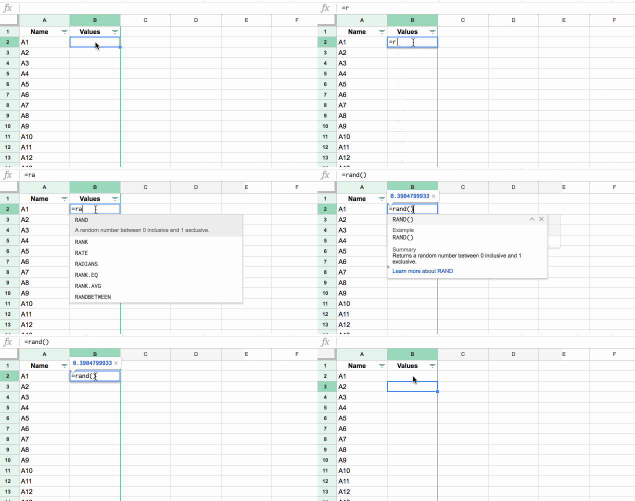
Your Google Sheet becomes unresponsive. This is the worse case scenario, and in my experience, if this doesn’t resolve fairly quickly, you don’t often recover from here.
So if you see this error message, and you’ve waited a few minutes but nothing’s happening, then you might want to just bite the bullet, exit the page, and pickup again but trying a different approach this time.
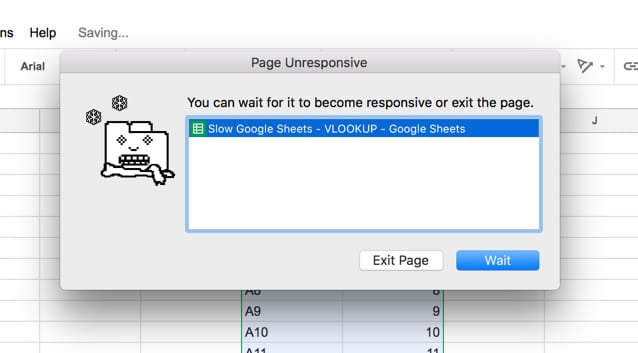
This is usually accompanied by your computer going into overdrive with the fan whirring loudly!
 2. Know the size limits of slow Google Sheets
Obviously if you’re dealing with large Google Sheets — Google Sheets with large amounts of data and/or formulas — then you’re more likely to see your performance suffer.
No discussion of slow Google Sheets therefore, would be complete without first discussing the size limits of Google Sheets.
Overall limit:
Google Sheets has a limit of 10 million cells per workbook (see Google file sizes).
If you do something that will take you past this limit (e.g. adding new rows or a new Sheet), you’ll see this error message:

Column limit:
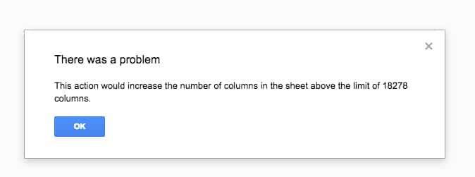
Google Sheets has a maximum number of columns of 18,278 columns.
If you do something that would take you past this limit, you’ll see the following error message:
Individual cell-size limit
Within a single cell, there’s a maximum string length of 50,000 characters (enough for approximately 500 average sentences, or about 162 Tolstoy sentences).
If you do something that would take you past this limit, you’ll see the following error message:

 3. Measure a Google Sheet’s size
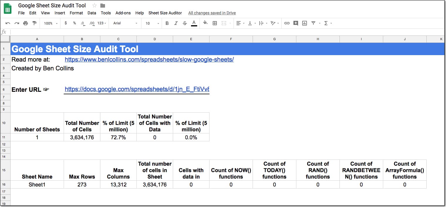
Using Apps Script, you can quickly build a simple tool to calculate the size of your Sheet.
This Sheets audit tool shows the total number of cells in the Sheet, how many have data in them and then statistics for each individual sheet too, including how many volatile and array functions you have (CLICK TO ENLARGE):
The code for this tool can also be found here on GitHub if you prefer.
I’ll do a post in the future looking specifically at how I built this tool with Apps Script.
New to Apps Script? Check out my beginner guide to Apps Script.
So that’s measuring the size of Google Sheets, what about measuring their speed?
 4. Measure a Google Sheet’s calculation speed
To measure the “speed” of various calculations you can make use of Chrome’s Developer Tools.
In your browser window, you can access the Developer Toolkit by pressing Cmd + Option + I on a Mac or Ctrl + Shift + I (on a PC). It can also be accessed in the View > Developer menu.
Under the Performance tab of the Developer Tools you can record the webpage (or Google Sheet in this case) as it loads, and check the screenshots box to show you what is happening and when.
For formula calculations, you can identify when the calculations start, e.g. marked by the 1 in this image, at around the 3.6 seconds mark:
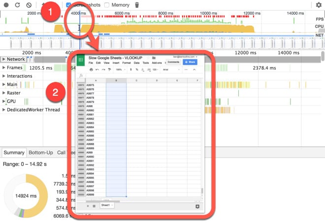
The number 2 shows a screenshot at this point in time, so you can see that your formulas are not showing yet.
You can identify when the formulas have finished calculating (the red box, around the 8.6 seconds mark):
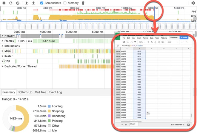
Check the screenshot to see that the formula results are showing in the cells now.
And so you an see how long this batch of formulas took to calculate:
8.6s – 3.6s = 5s
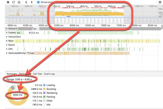
There’s a whole lot more to the Developer Tools, but that’ll do us for today.
This is the methodology I’ve used to calculate formula speeds for comparison tests. I ran all of the tests in the same place at the same time of day (so wifi speed discrepancies were negligible) and also ran them each multiple times and took averages.
 5. Delete un-used cells
Your Google Sheets will get slower as they get larger.
So one of the first things to try, before getting into the marginal gains of formula optimization, is reduce the size of your Google Sheet.
Blank cells slow down performance, dramatically so in fact. So it’s a good idea to delete them whenever you can, so you reduce the number of cells Google Sheets is holding in memory.
Ideally you should remove any large numbers of blank rows under your datasets, or columns to the right of your datasets.
What about new rows being added automatically?
Don’t worry if your data is being imported automatically by Apps Script or a third party tool like Supermetrics or Tiller, as the new rows are automatically added to your Sheet as required.
(However, you should always test this theory with your specific setup or app, to confirm this is the case.)
 6. Convert formulas to static values wherever possible
Once you’ve used a set of formulas in your data, and you’re sure you won’t need them again, you should convert them to values.
This should reduce the file size, which will help performance overall, and it’s also best practice (to reduce errors occurring if someone or something happens to break the formulas).
You change formulas to values by copying them and then:
Edit > Paste special > Paste values
Better yet, learn the keyboard shortcut to save yourself time. Highlight the formulas to change, Ctrl + C on a PC or Cmd + C on a Mac to copy and then Ctrl + Shift + V on a PC or Cmd + Shift + V on a Mac to paste as values.
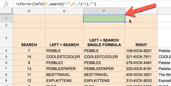
Note, I advocate keeping a copy of a “live” formula at the top of your columns of data in your tables, so you have a record of how the calculation was performed and can also very quickly re-use it if needed:
 7. Use closed range references
Closed range references means using something like A1:B1000 instead of A:B in your formulas (i.e. you explicitly specify the boundaries of your range).
If you’re working with large Sheets and are using open references where you don’t need to, this will be adding extra calculation overhead to your Sheet.
It might not look like there’s much data in column A, but Sheets will check every cell, including all the blank ones, if you use open ranges like A:B.
Note: Whilst this is generally a good idea for speeding up your formulas, there are obviously situations when an open reference is desirable, for example when new data is anticipated. Leaving an open range will allow any new data to be included in calculations.
 8. Remove volatile functions or use with caution
In Google Sheets there are four functions, NOW function, TODAY function, RAND function, and RANDBETWEEN() function, that are known as volatile functions, which means they recalculate every time there’s a change to the Sheet. All dependent formulas must also be recalculated too (i.e. formulas that reference or include a nested volatile function).
This uses up processing power and so can negatively impact your Sheet’s performance, although this is only going to be noticeable if you have large numbers of them.
To illustrate, I copied 100,000 TODAY() functions down column A, which took my machine about 5.5 seconds.
I then deleted 99,999 of these formulas and just left TODAY() in cell A1 and then put the following formula in cell A2:
= $A$1and then copied this one down. The dollar signs represent absolute references and keep all my formulas locked onto cell A1.
Running this formula down 100,000 cells in column A took around 4.1 seconds, so almost 1.5 seconds quicker.
It’s also best practice to do this, because if I ever need to make a change to the date, then I can just change it in this one place, A1, and not have to redo all of my formulas.
 9. Vlookup strategies
To improve the performance of your VLOOKUP formulas in Google Sheets, use closed, rather than open, range references for your search tables where possible (see no. 7 above).
Reduce the size of your lookup table, if possible, although this only has a marginal positive effect in my experience. For example, rather than search across everything you might use the Filter function to create a smaller, helper table for the lookup first, and then use that in your VLOOKUP (see no. 17 below).
However, don’t be tempted to nest other functions inside your VLOOKUP and create the table on the fly each time. It’s much, much slower.
For example, this formula is bad practice and will really slow down your Sheet if you have a lot of them:
=VLOOKUP( $A1 , UNIQUE( FILTER( $K$1:$N$10000 , $K$1:$K$10000 < 100 )) , 2 , FALSE )whereas creating that nested Filter table as a helper table and referencing it is the preferred method:
=VLOOKUP( $A1 , $F$1:$I$10 , 2 , FALSE)Combining VLOOKUPs with Array Formulas to return multiple column values with a single lookup is significantly slower than simply using multiple individual VLOOKUPs.
In Excel, sorting your data and using approximate matching (TRUE as your final argument in the VLOOKUP) is quite a bit faster than the exact matching algorithm (FALSE as the final argument). It’s slightly quicker in Google Sheets too, but only slightly it seems, so it’s not worth the extra hassle.
Another Excel VLOOKUP trick is to use two approximate matching VLOOKUPs instead of a single exact match. It’s significantly faster because the underlying search algorithm is much, much faster. However, I found this technique was actually slightly slower on Google Sheets so I wouldn’t recommend it.
 10. Index-Match strategies
The Index-Match is a powerful lookup combination and well worth learning (learn it in day 10 of my free Advanced Formulas 30 Day Challenge course).
In its classic construction, you might see formulas like this:
=INDEX( Sheet2!$A$2:$P$51 , MATCH($A3,Sheet2!$G$2:$G$51,0) , MATCH(C$1,Sheet2!$A$1:$P$1,0) )where you have two nested MATCH functions to lookup the row and column numbers (which is why index-match-match is so flexible).
This is fine for small numbers of index-match-match formulas, but inefficient at scale.
Say you’re looking up 10,000 rows and 10 columns. For every single cell, you’re using two matches to lookup the row number and the column number, so your total number of calculations would be:
No. of Match functions for row +

No. of Match functions for column +

Index Match function =
(10,000 rows * 10 matches) +
(10,000 rows * 10 matches) +
(10,000 rows * 10 indexes) =
300,000 calculations
Much better to split the match lookups out into their own helper row and column rows, as shown in this example:
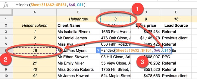
By splitting both the match lookups into their own row and column, you can compute them all once first, and then use those numbers in your index function.
Now you’ll only have to calculate the index function when you do your calculation, so your total calculations now would be:
(10,000 matches for the rows) +

(10 matches for the columns) +

(10,000 * 10 indexes) =
110,010 calculations
Significantly less than before, only about 1/3 as many calculations to do!
 11. Query function strategies for slow Google Sheets
As alluded to above , using open range references can hurt performance because you may inadvertently include thousands of extra blank rows in your calculations (see no. 7 above).
Instead, use closed range references or create smaller helper tables as inputs to your Query functions to speed up performance.
For example, running tests with a QUERY function, I found that each additional 20,000 empty rows I was including with open ranges would add 1 second to the calculations.
So rather than a formula like this for example:
=QUERY( Sheet2!A:E , "select *" , 1 )you’d be better served by specifying the range explicitly:
=QUERY( Sheet2!A1:E100000 , "select *" , 1 )This improves the Query function speed because the calculation is no longer including all of the blank rows in Sheet 2 under the dataset.
 12. Array Formula strategies
If you spend long enough reading help forums you’ll find people saying that using a single array formula to replace hundreds of individual formulas will be quicker, and others staunchly saying the opposite. So which is it?
In my experience, array formulas working on big datasets (those with lots of rows) are slow and will make your Sheet sluggish. I’ve found they tend to be slower than the individual formulas.
However, they’re so useful in specific situations, like gathering Google Form data, that I still recommend learning about them and using them, with caution.
I use them heavily for performing running calculations on datasets that grow over time (new rows being added). That way I know the calculation happens without me needing to update anything.
For example, this formula:
=ArrayFormula( IF( A2:A <> "" , A2:A * 100 , "" ))which is the array version of this individual formula:
= IF( A2 <> "" , A2 * 100 , "" )will automatically compute a value for every new row of data added.
I would test both versions on your own sheets, and choose whichever is most appropriate (weigh up speed versus array benefits of automatic calculation). The individual formula approach has the added benefit of being easier to debug and setup.
If you want to keep array formulas (and I hear ya!) consider archiving historic data periodically (see no. 21 below), to keep the live dataset manageable.
 13. Import Formula strategies for slow Google Sheets
The ImportHtml function, ImportFeed function, ImportData function, ImportXml function, and ImportRange function pull data from sources external to your Google Sheet, so they require an Internet connection to function.
They’re slower than other functions that operate entirely within your single Sheet, so they will potentially affect the performance of your Sheet.
For example, using IMPORTRANGE to import large amounts of data from another Sheet will take time and you may see the Loading… error message for a while:
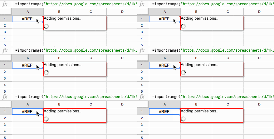
The IMPORTRANGE is a slow formula because it’s connecting to another Sheet to retrieve data. In general, it’s best to minimize the number of these external calls required.
However, when your data starts to get really big (around 20,000 rows), the IMPORTRANGE formula will just get stuck at the Error Loading data... stage.
In this case, use multiple IMPORTRANGE calls to retrieve your data.
Combine them into a single formula using the { ... ; ... } array notation, for example in this formula which gets the first 15,000 rows and then the next 15,000 (up to 30,000) from Sheet 1 of our source Sheet:
={ IMPORTRANGE("https://docs.google.com/spreadsheets/d/1UrtOONA8B2pNYCI1byDA__R9_Bbz0GWrfxP_MDotaTY/edit#gid=1789207765","Sheet1!A1:E15000") ;

IMPORTRANGE("https://docs.google.com/spreadsheets/d/1UrtOONA8B2pNYCI1byDA__R9_Bbz0GWrfxP_MDotaTY/edit#gid=1789207765","Sheet1!A15001:E30000") }
Other Notes
Note, you’re limited to a maximum of 50 of ImportData functions in a single spreadsheet (link).
None of the other Import formulas have an explicit limit like this on their help pages and some limited testing suggests that if there are any limits, they’re certainly greater than 50.
By default, these functions recalculate as follows (see documentation):
- ImportRange: Every 30 minutes
- ImportHtml, ImportFeed, ImportData, ImportXml: Every hour
 14. Google Finance Function strategies
The GoogleFinance function is another function that retrieves data from an external source, so requires an internet connection. Like the Import formulas above, it will be slower than regular functions operating inside your Sheet only.
Again, the general strategy here is to reduce the number of external calls you make with GoogleFinance function, i.e reduce the number of GoogleFinance functions you use.
So think about retrieving a whole year of stock prices with a single formula, rather than hundreds of daily functions for example.
Per the documentation, GoogleFinance data may be delayed up to 20 minutes.
 15. Use IF statements to manage formula calls
You can use an IF function wrapper to check whether a calculation needs to be performed before doing it.
Example
Say for example you have a table of product data that includes books, and you want to use a VLOOKUP function to bring in book sales data alongside each book.
So you set your VLOOKUP up to search for the ISBN number (the book’s serial number) in the sales data table and return the sales value. The inefficiency comes because you’re searching for all your products, not just books, so all those products that have N/a in the ISBN column are still be searched for.
Instead, check first for the ISBN number and then only perform the lookup if you have a valid ISBN.
The formula could look something like this, where you first check that the ISBN lookup value is not equal to N/a:
= IF( A2 <> "N/a", your_vlookup , "Not a book")or more generally:
= IF( test , calculation_if_test_true , output_message_no_calc ) 16. Manage expensive formulas with a control switch in slow Google Sheets
Use a control switch cell with the IF statement method from above, to keep things manageable.
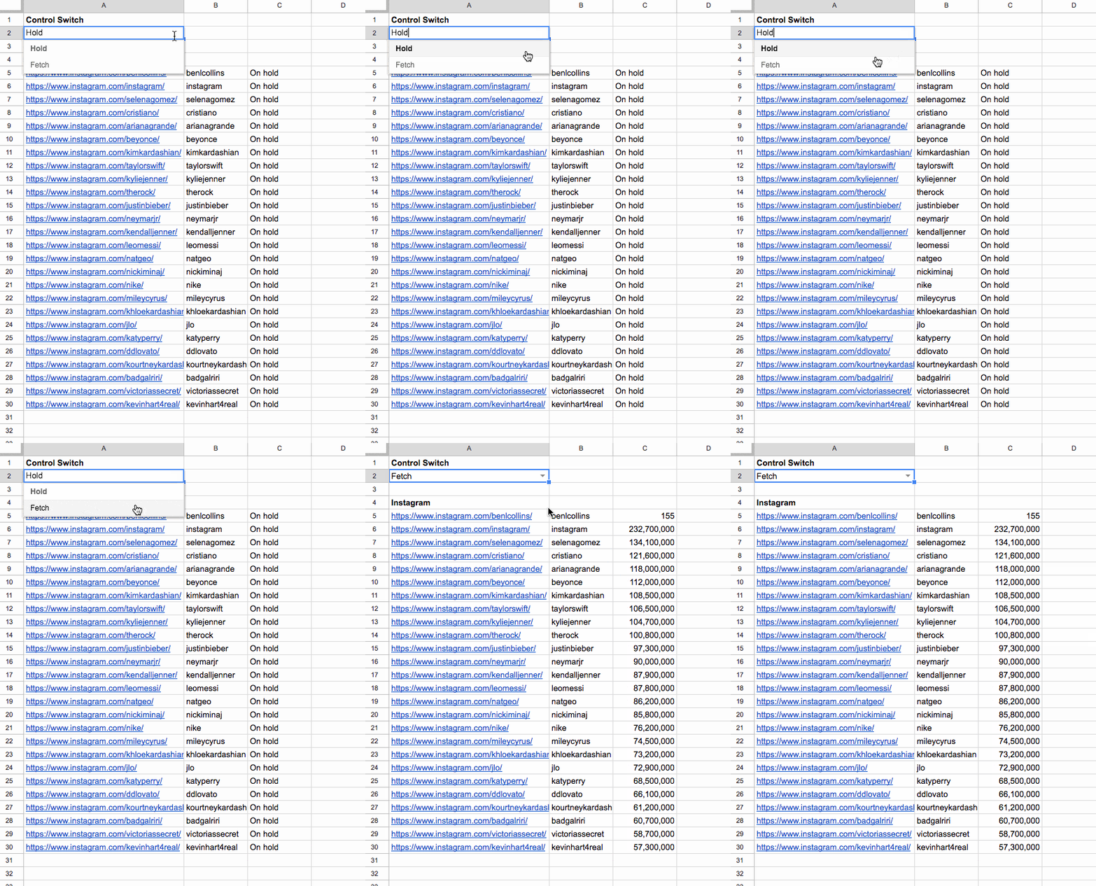
Use data validation to create a drop-down menu in a single cell, the control cell, with values “Process” and “On Hold” (or whatever makes sense for you).
Then use an IF formula like this to only process the performance-hungry formulas in your slow Google Sheets when you want to:
=IF( $A$2 = "On Hold" , "On hold" , your_formula_here )Here’s an example of this control switch technique applied to some performance-hungry Instagram IMPORTXML formulas (for the top 25 accounts):
 17. Use Filter, Unique and Array_Constrain functions to create smaller helper tables
The Filter function, Unique function and Array_Constrain function all accept ranges (tables) as inputs and return ranges (tables) as outputs, that are smaller than the input tables.
Thus they are useful to create helper tables for further data analysis work.
Say you had a table with 100,000 rows of data in, but were only interested in performing calculations on a subset of that data, then you could use one or more of these functions to reduce the size of your table and create a new helper table for your calculations.
For example, you might use the Filter and Unique functions to create a helper table from a dynamic subset of your larger table:
=UNIQUE( FILTER( A1:E100000 , B1:B100000 < 100 ))or using Array_Constrain to create a helper table from a static subset of your larger table:
=ARRAY_CONSTRAIN( A1:E100000 , 10 , 4 ) 18. Avoid Long Calculation Chains
By long calculation chains, I mean cells that reference each other in a long chain, for example a long column of cells equal to the cell above, like so:
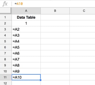
I created a column with 100,000 copies of this formula, referencing the cell above, and it was NEVER able to show all of the formula answers, even though the underlying formulas were showing in the cells.
I had to close the file, wait a moment and re-open to see the completed results.
Interestingly, this blank cell issue always occurred at the 99,100 occurrence of the formula. Here you can see the formula referencing the cell above (A99102) but not showing the value 1 like the cells above are showing:
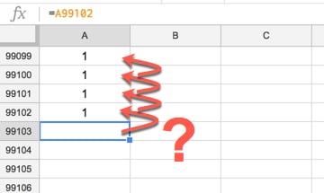
(I hit this 99,100 limit in all the various chaining tests I did, which makes me think it’s some kind of limit to what Sheets can handle for linked cell calculations.)
It’s slow and may not even complete the calculation under certain conditions.
Aside from that, it’s also very bad practice to chain calculations like this. One error will cascade through the entire chain and it’s also difficult to debug.
A better practice would be to reference a single cell with absolute references and then copy that down your column, e.g.
= $A$2 19. Reference data on the same Sheet
Referencing data in the same sheet keeps things simple — always a good practice — and saves time because your formulas can access the data more quickly.
Obviously it’s not always practical or convenient to reference data in the same tab of your Google Sheet, but keeping references within your one file will be quicker than using IMPORTRANGE to bring in data form other Google Sheet files.
That said, below I discuss the pros of splitting up large, slow Google Sheets (see no. 21 below) and using IMPORTRANGE to bring them back together as necessary.
 20. Use helper columns
Tempting as it is to create clever formulas that do everything in one go, there are many advantages to creating helper columns. Not only are they easier to create, they’re easier to follow (for you and colleagues), easier to debug, and they can even be faster sometimes too.
Suppose you have a list of a website’s URLs in column A and you want to quickly extract the path, the part of the URL after the www.website.com address.
You might use this formula in column B:
=RIGHT( A1 , LEN(A1) - SEARCH( ".com" , A1 ) - 4 )Now, since the hostname is the same in each case in this example, we’re needlessly calculating the nested SEARCH function every time.
We could run this once, figure out that our hostname was 24 characters long (and store this in a helper column to ensure best practices), and then replace the SEARCH function with this constant ( 24 digits + 4 digits for the “.com”):
=RIGHT( A1 , LEN(A1) - 28 ) 21. Split your slow Google Sheet into separate Sheets
First of all, it may be time to consider warehousing your data in a proper database and not Google Sheets if you are getting close to that 10 million limit (see no. 27 below).
Assuming we’re sticking with Google Sheets though, it might be time to split up your huge dataset into separate Sheets if your Sheet is so slow that it’s frustrating to use.
This technique should be approached with CAUTION though, to avoid data loss. Only do this if you’re confident you know what you’re doing and you’re sure you really need to.
Be aware that this approach comes with a cost also. Before you had one single table to keep track of, to modify, update and analyze, whereas now, if you split it up, you’ll need to keep track of multiple Sheets and ensure that changes and analysis are consistent.
A safe bet for this approach might be to offload prior years of data say, or old products that are no longer in your inventory. In other words, it’s data we don’t envisage using again, but that we want to keep a copy of.
How to safely split up slow Google Sheets
The best approach to split up your really big Google Sheets is to make new copies, label each Sheet clearly and then delete all the data apart from the data relevant to that Sheet. For example, if you’re offloading data from 2015 into its own Sheet, then here are the steps:
- Make a copy of the master Sheet, with all your data in
- Name this new Sheet and include “2015” somewhere in the title
- Sort the data by year in this new Sheet
- Add a filter and show everything except 2015 data (i.e. hide the 2015 data)
- Delete all these rows
- Remove the filter to leave only the 2015 data
Once you’ve completed all the steps for all your archived data, you’ll want to remove it from your master Sheet. I’d advocate keeping a full copy of your master Sheet before you start deleting any rows of data though.
You’ll end up with a master Sheet that just has your current, or live, data in it, and it’ll hopefully be much faster.
You can also do any calculations or data analysis locally and then bring the data back together in your master Sheet using the IMPORTRANGE formula.
 22. Use Conditional Formatting sparingly
Conditional formatting is a super nice feature for adding extra context to your Google Sheets, for example highlighting outliers or values above thresholds. I use a lot in my scheduling sheets to highlight the row for the current day for example.
However, it can be very slow on large datasets because it’s implemented on a cell-by-cell basis.
So it’s best used for small data tables and in your presentation tables and dashboard reports.
 23. Leverage the power of Apps Script on slow Google Sheets
Apps Script is a Javascript based scripting language that can be used to extend the functionality of Sheets (and interact with other Google services). Check out this Beginner Guide to Apps Script if you’re new to it.
The possibilities here are extremely broad, encompassing everything from automating repetitive processes to speed up your workflow to creating custom functions to save you typing out complex formulas over and over (see next section).
Apps Script is extremely effective at doing big batches of calculations, especially repetitive ones, often more quickly than thousands of regular formulas.
Example
Imagine I have a column of numbers that I want to classify into Small, Medium and Large using a nested IF statement like this:
=IF( A1 > 500 , "Large" , IF( A1 > 250 , "Medium" , "Small" ))This took about 6.5s to compute for 100,000 rows, and about another 30s to copy and paste as values (another best practice for optimizing your slow Google Sheets – see no. 6 above).
Replacing this with Apps Script and running for the same data range took around 16s to paste in all 100,000 values, so less than half the time.
Here’s the code for this function:
function columnClassifier() {

  var ss = SpreadsheetApp.getActiveSpreadsheet();
  var sheet = ss.getActiveSheet();
  var input = sheet.getRange(1, 1, sheet.getLastRow(), 1).getValues();
  var output = [];

  for (var i = 0; i < input.length; i++) { if (input[i][0] > 500) { output.push(["Large"]) }
    else if (input[i][0] > 250) { output.push(["Medium"]) }
    else { output.push(["Small"]) };
  }
  sheet.getRange(1,2,output.length,1).setValues(output);
}
Optimizing your Apps Script code is an entirely different and gigantic topic in its own right, so I won’t make any comments in this article. Note however, the current quotas and limitations applied to Apps Script code.
 24. Use custom formulas sparingly
Custom formulas, also known as user defined functions, or UDFs, are custom functions written in the Apps Script script editor window.
Complex custom formulas will be very slow if you approach them in the traditional function way, and read/write single cells at a time.
For example, consider this custom formula to mark up a product price by 15%:
/**
 * Markup a price by 15%
 *
 * @param {number} input The value to markup
 * @return The input multiplied by 1.15.
 * @customfunction
 */
function MARKUP(input) {
  return input * 1.15;
}
which looks like this in use:
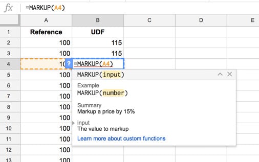
Copying and pasting this down 1,000 rows is SUPER slow. It took me about 10 seconds, but it’s also dependent on your wifi connection.
What you need to do with custom formulas, to improve their performance, is think more like array formulas. The slow part of these formulas is the reading from, and writing to, the Sheet, as this happens via the spreadsheet API, so it’s dependent on your wifi connection.
It’s best to minimize the number of read/write calls to your Sheet if you can.
Say you want to perform a calculation on 10,000 cells, then you’ll be better off reading all 10k cells into your function once, performing the calculation and then outputting back to your Sheet in one go, as a range.
For example, change the above formula to this more general one, which accepts a range input and outputs a similar sized range:
/**
 * Markup a price by 15%
 *
 * @param {number} input The value or range to markup
 * @return The input multiplied by 1.15.
 * @customfunction
 */
function MARKUP_RANGE(input) {
  if (input.map) {
    return input.map(MARKUP_RANGE);
  }
  else {
    return input * 1.15;
  }
}
This will perform the same calculation on 1,000 cells in under a second, which is significantly faster. This is how it works in practice, accepting the whole range as the input now:
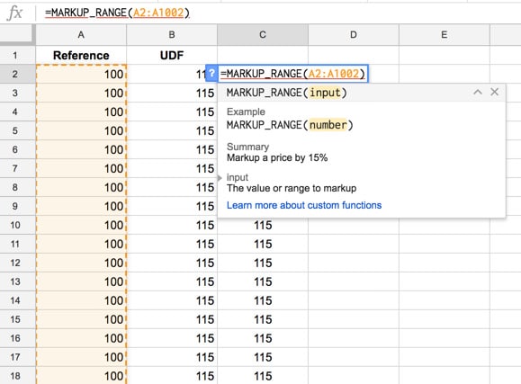
Note: Custom apps script formulas are recalculated only when their arguments change. Also, these arguments must be deterministic, i.e. not one of the volatile functions like NOW() or RAND(). If your custom function tries to return a value based on one of these, it will display Loading... indefinitely.
Read more about custom function optimization on the Google documentation.
 25. Other troubleshooting tips for slow Google Sheets
Sometimes it might not be an issue with Google Sheets that’s causing the slow response time. It’s worth trying these strategies to see if any resolve your issues:
> Close and re-open the Google Sheet (sometimes it’s the simplest fixes that work).
> Refresh your browser.
> Clear your cache and cookies.
> Try another browser or operating system. Make sure both browser and operating system are currently running on their latest version.
> Disable browser plugins or extensions.
> If possible, try replicating the issue on another computer to see if it’s the computer hardware having issues. A Google Sheet’s calculation speed depends mostly on the local resources.
> Try replicating your issue on another wifi network to see if it is a network issue. Most functions are run locally in the browser but some, like the IMPORT formulas, require access to the Internet (as well as any Apps Script which is run on Google servers).
> Try disabling and re-enabling offline access.
> Try a faster computer perhaps ¯\_(ツ)_/¯
 26. Understand changes in the cloud take time to propagate
Remember that if you’re working in real-time with other collaborators, changes can take a few moments to synchronize.
Other users and any apps script files will be seeing a cached version of the Sheet until all the synchronization operations are completed, and this may affect how certain cells appear. For example, they may well have finished calculating in your Sheet but still be showing blank or #N/A in the view a collaborator sees.
Just something to keep in mind, and honestly, it’s a very minor point. In my experience it all happens so quickly that it does feel almost instantaneous, although again really large, slow Google Sheets will suffer from this more.
 27. Know when it’s time to move to a database
There will come a time, and perhaps you’re already there, when you have to admit defeat and accept that Google Sheets won’t fulfill all of your data needs. For all of its strengths, of which there are many, that 10 million cell limit fills up pretty quickly with real-world data.
Well before any of your production Sheets approach the 10 million limit you should think through the next steps beyond slow Google Sheets.
You’re going to want to move your data into a database archive. You can still work in a Sheets environment but offload the data storage to a dedicated database.
Google Database Options
Within the Google ecosystem, we’re talking about BigQuery and Cloud SQL, both cloud databases. However, the integration isn’t simply drag-and-drop anymore, so you’ll need development skills to connect these services.
I’ve written a guide to help you get started with Google BigQuery:
Beyond Sheets: Get Started With Google BigQuery
With your data in BigQuery, enterprise level Google Workspace accounts can use Connected Sheets to analyze that data, even if it has millions of rows!
 Conclusion
That’s all folks!
I’ve tried to make this post as exhaustive and as useful as possible, but I’m absolutely sure there are more ideas out there.
I welcome any comments and thoughts on this topic. Think of this post as a living, breathing article to which more will hopefully be added in the future.
Thanks for reading and I hope the insights contained herein have been valuable!
(This post contains some affiliate links, which means I earn a small commission on any signups for the products mentioned in this post. I only do this with products I personally use and believe in.)

Great stuff Ben, thank you! Will refer to this article often, both for my own sheets, and in support of users on the Sheets Help Forum.
That “Toggle” idea btw is great. I’ve got a sheet on which, in addition to a the primary duties the sheet performs, there are many tabs that show reports that are only occasionally needed. Since these reports Query or Filter the entire database, I don’t want them running in the background when the user is not even looking. I put a giant ON (in green) / OFF (in red) switch cell at the top of the report, keeping them deactivated when not in use.
Lots to think about here, and I’m going to flip through the structure of my sheets looking for opportunities to apply these ideas. Great stuff Ben!
Best,
Lance
Thanks Lance! Great to hear of your use case for a toggle switch too. Let me know if you have anything to add 😉
Great info! I have a sheet that you to 100 people at a time are recording info on (a daily tracker type thing) and as I got over 60, many noticed their phones kept crashing or not loading the sheet. It also seemed to coincide with the month I added some ArrayFormulas and Queries (within the sheet) to the mix.
Any advice on creating a simpler interface while having calc a going on I t he background so mobile users don’t get the shaft? I can send you a link to the sheet if you want, but I’d rather not post on public forum.
Brian, you ever figure this one out? My company is using sheets and those using their ios devices have had their sheets app crashing constantly particularly on sheets with a lot of import ranges and array formulas.
Hi Ian – you might want to check out OnPlan.co . We can act as a bridge between two google sheets models. Most people use us for financial modeling – but would like to understand more about your use case.
Ben,
Brilliant! A very timely article as I attempt to speed up my unwieldy sales tracking spreadsheet. Lots of great ideas to implement!
Thank You!
Bernie
Thanks Bernie!
Thank you Ben, super useful and very helpful information. This post will certainly be part of my “G Sheets how-to reference manual”.
Keep up the great work , looking forward to seeing more advanced Google Script how-to´s and courses!
Cheers,
Thanks Frank!
Great Article Ben.
Thanx for such an exhaustive article. I was indeed looking for such article for some time.
Just a question: Somewhere I read that there is a limitation of number of formula cells to 40,000. I am already have a sheet having more than this so this limit is definitely not correct. But is there actally any limit on the number of formula cells or the only limit is overall number of cells limited to 2 million?
Further is there any script that removes unwanted rows and columns from the sheet?
Yes, that must be an old limit, but it doesn’t exist now. I’ve not heard of a formula cell limit anymore, but I’ll add it in here if I do. For deleting rows you could try this add-on: https://chrome.google.com/webstore/detail/remove-blank-rows-and-mor/gmidogdphchbiehdmbigdbcopkpjpnio?hl=en-US
You could quite easily write a small script to do it yourself too. You’d need to calculate the max rows and the last row with content and then delete those rows.
Hope that helps!
Ben
Dear Ben,
Thanx for the reply.
As you said in the article, I have also observed that normal formulas are speedier than array formulas but then formulas need to be copied every time new rows are added.
To reduce the work I have developed a small script which adds row and then copies the formulas formulas in the new rows. But for each sheet I have to make changes in the script to remove the values from non-formula cells depending on the requirement.
I have not been not able to develop any generic formula that can be used in different sheets.
Can you suggest some way to copy only from formula cells or copy all but then remove values from all non-formula cells.
The script used in one of the sheet is given below:
function AddRows_FOR_sheet() {
var sh = SpreadsheetApp.getActiveSheet();
var s = sh.getActiveRange();
var row_position = s.getRowIndex();
var row_num = Browser.inputBox(‘Adding row below current position’, ‘Enter row numbers to be added’, Browser.Buttons.OK_CANCEL);
var lCol = sh.getLastColumn();
sh.insertRowsAfter(row_position, row_num);
var range = sh.getRange(row_position, 1, 1, lCol);
range.copyTo(sh.getRange(row_position + 1, 1, row_num, lCol), {contentsOnly : false});
}
Perfect! Very relevant! Impressive!
Thanks !
Thanks Sergei
Thanks Ben!!
seriously awesome tips.
Now, i can easily speed up my google sheet and my productivity also.
thanks for posting for us
and save our valuable time in future
Thanks Nitish
Thank you Ben, that’s an awesome post, coming right on time, and tips which are not in many other places.
Thanks Cédric!
Ben,
What would you recommend for hardware to make the sheets calculate as fast as possible. An i7 K series processor? or xeon? have you tried different hardware?
Jason
Once again, trying to get a copy of Google Sheet Audit Tool. But the link download never sent to my email. Also for another similar link in this website since along time ago.
I always end up for giving up when face situation like this in this website.
If you really want to share, why you make it more difficult?
or do you actually just want to grab other people email only or do you just want to attract people to visit your site?
otherwise, you better not share it buddy rather than giving a fake link to readers
Hi Dave,
Sorry you never received the template email (maybe in your Spam folder?). I just tested the link and download email and it’s appears to be working fine. Have sent you the template email directly in any case!
Cheers,
Ben
Hi Ben
Thank you for your sheet link.
Sure, i’ve checked before in my mail folder including spam folder and there is no mail response from your submitted link in your website
Now i receive it after you sent it manually.
Hi Ben.
Thanks for this great article. It was very helpful!
I’m having an issue with one of the spreadsheets I use. It has a large amount of data, some scripts and IMPORTRANGES, but it’s still usable.
What’s the problem: when I edit (add or delete data) from one specific column in one specific sheet, the formula calculation bar starts to load and keep loading for a long time. It also “breaks” the IMPORTRANGE formulas from other spreadsheets that link to this “problematic” spreadsheet.
The input data from this column triggers only an VLOOKUP formula in the cell adjacent to it. The are other features in the spreadsheet that are way more complex ant this doesn’t occur when editing them.
Have you seen anything like it? Do you have any idea what that might be?
Cheers,
Italo.
Thanks! This is awesome! Is Google Sheets faster with a business G Suite account versus a free personal Google account?
I’ve followed the advice in several of the items here, and they did help considerably, but it can still take 10 seconds to recalculate when a user makes a change to a single value on one of the tabs in their spreadsheet. The formulas are very simple. There are no vlookups and no importranges or anything like that. But there are 32 tabs with anywhere from 50 to 300 similar rows. It’s almost as though Google Sheets is recalculating all 32 tabs when it isn’t necessary.
Is there a way of toggling autocalculate on and off? Perhaps there’s an add-in that will turn off autocalculate and let users recalculate on demand. I don’t know what to do, but waiting 10 seconds for each simple change is getting to be too much for the people using this sheet.
Any further suggestions at this point?
Hi Ben,
great article, however i don’t see much info about how to improve the importxml function.
Does-it exist a function which allow us to store the data and not check again and again, maybe juste once a week ?
Because i try to check regulary (one a week/month) if links are still on webpage. But it’s so slow on Spreadsheet and sometimes it just fail.
Excellent
Can you backup your claim that array formulas are slower than individual formulas? The strategy used to time the sheet and the actual sheet used, the actual formula used, the number of times, You’ve repeated these tests?
Thanks for your tips. But In Google Sheet Audit Toll after aproximately 5 minutes running script in my google sheets, show this message: Exceeded maximum execution time
My spreadsheet is extremely large, I believe there is not enough time for the script to run. Here are some suggestions to work around this kind of problem: https://stackoverflow.com/questions/7854573/exceeded-maximum-execution-time-in-google-apps-script
I posted this issue in github: https://github.com/benlcollins/apps_script/issues/1
Unfortunately I am not aware with codes to try to fix this problem 🙁
Thanks
I discovered that what was making my worksheet slow was a PivotTable where I processed my entire data table. I removed the PivotTable (which I use exporadically – about once every 2 months), when I need to use it I create a new one at the time of need as it was just to sort the data.
Good evening,
I’ve added your script to my Google docs library, given all the auth but it keeps saying “Please enter a valid Google Sheets URL”
I’ve just done a copy/paste on your cell B6 of the whole URL of my google sheet doc… Where I’m failing? 🙁
Hi Marco,
This sounds like a permissions issue. You’ll need to ensure the Audit Sheet account has read access to the file you want to check, otherwise you’ll get that error. You can go into your google doc sheet and share it with the same Google account where the audit file is.
Hope that helps!
Ben
Hello Ben,
I’ve multiple spreadsheet but it’s the only one giving me this error…
Is it possible to share that one with you so you can double check?
Sure, you can share with me at ben [at] benlcollins.com and I’ll take a look if I can find the time.
Done, than you so much. The file name is Financial Resume 6.1. I’ll write inside my email so we can have a direct contact.
Thank you indeed 🙂
Hi Ben,
I can find where to send fresh comment , request you to please help me to resolve the issue, my spreadsheet is being used by my team and every morning my actual time column which is filled by team gets automatically changed at around 9:30 and all enteries based on actual time and date gets changed to current time (means 9;30 and the time)dont know why , hope i am clear to u.
Great article! Now I understand better a lot of points of the performance of Google sheets.
Thanks!!
How I can use the chart in various way in google sheets as i want to see a month selling of my products
Hi Ben,
thank your for the great article. Very informative!
I have a question. On the office we work a lot with a Google Sheet that has about 5 tabs. Usually 3 of us work on it simultaniously. And others, also on other locoations, have the page open.
Sometimes the page gets pretty slow.
Does working like that affects the speed of Google Sheets?
Would a reload help?
Regards, Felix
Excellent article. My problem is strange though. When I type a new formula and hit “Enter” the cell does not show the result until I perform a change in another cell (even though I can see the formula if I leave and come back to the cell). Once I have made a change in another cell….. entering a single character then hitting “Enter” for example, the formula’s result appears in the original cell. Happens on a variety of devices (All Win 10 running Internet Explorer OR Chrome and on any Ethernet/WiFi network). Any thoughts?
Thanks for the work on this article. Ben do you know how upgrading your computer will affect Google Sheets, meaning which has a better effect more memory or a faster CPU. Of course help but could you shed any light on the subject.
Thanks
In the case of a large index+match table, do you think it would also be faster to use a double filter? You could do:
=filter(filter(table,column=value),row=value)
Or is it possible to use getpivotdata on a table that isn’t actually a pivot table?
Hi Ben, awesome article!
I have some questions related to the loading-times workings of IMPORTRANGE.
A.
Lets say I have one “source” file with a large database.
If I call on that database in another file but filter the importrange:
filter(importrange( [url], “A:E”), A=”[value]”)
does it import everything first and then apply the filter locally, or does it apply the filter and then only import the filtered data? ie, is the importing process faster if it’s filtered?
B.
If I have 3 different sheets and import their data into one “source” sheet with from which my employees’ individual sheets import their filtered data.
When the individual employee sheets call on the one “combied” source sheet, does it take longer because in the backend it needs to gather from the other 3 source sheets? Or is that all instant in Google’s cloud backend?
Great article with a lot of helpful hints! Didn’t know about the ArrayFormula wrapped in the VLookup to return values in multiple cells instead of using multiple VLookup formulas. That is a great discovery! Thank you so much! I know you caution against using ArrayFormulas, but according to the worksheet audit page provided, I am using less than 5% of my available allotment. So any opportunity to program fewer formulas I will jump at!
Hi Ben, is the Google Sheet Size Audit Tool working? Because I made a copy and entered the URl of the spreadsheet I want to audit but nothing seems to happen…
Thanks
Hi Sebastian,
The tool is working fine. It took me some time to understand why it is not running from my end too. You need to open the Script Editor form Tool and then try to run the macro called “sheetAuditor” from menu “Run”. You will be prompted for authorization and once you allow the access to your files the data should load properly.
hey guys! I tried to copy paste and ran the script in the background after adding my URL but it doesn’t work 🙁 any recommendations? thanks
Delay from form submission to spreadsheet view of submission
Hello, great article, very helpful.
I am now experiencing a delay of 5-10 minutes from the point of form submission (the user hitting SUBMIT) to being viewable in the spreadsheet view. This happens sporadically, but when it happens it can takes 4 or 5 hours. I can not find the cause. I recently “cleaned” the form and the sheet, now are only 350 used rows with 17 columns.
Any suggestion please. Thank you very much
I have the following formula in a sheet:
=if(E1=”HOLD”,,query(Cust_Orders!B6:Z5000,”Select Y,G,I,H,K where H>0 “))
With E1 being a drop down with values HOLD and FETCH
The recalculation when I go to FETCH takes about 13 seconds.
But when it is in HOLD, the query doesn’t execute, and everything goes blank.
Not what I want.
I’m trying to avoid recalculating this query every time I make a change in the Cust_Orders range, but keep the old values, as two different pivot tables that are viewed by other people are dependent on it.
Is there a way to do this?
I have one more suggestion to offer to improve the speed if today() function is being used in a large number in a sheet. As we all know these formulae are volatile and with every change in the sheet they are recalculated. It definitely will slow the sheet.
Instead, if we create a range (say today), use it in formulae and update it just once in a day through a trigger, it avoids unnecessary recalculation with every change.
awesome tips. Been working on improving the speed of my sheets and some of my clients. Since we use our own custom add-on, there’s a lot of processing involved and shortening the time with these tips certainly help.
The control switch one is great since I’m working with volatile ecommerce data that is constantly refreshing. Could turn it into a button too.
Hi , my google speardsheet is troubleing me from last 15 days , i always need to paste as values before i leave office ,but after 6 pm untill morning 9:30 my all actual time and date cells are getting changed which are being filled by my team,and next day i need to fill all enteries manually . wha is the reason for this ,please help
I don’t know why but exporting data from ‘heavy’ sheets into csv-files, deleting those sheets, making new sheets and importing the data into those new sheets helps a lot.
Thanks Mariette , We delete data from google sheet very frequently ,like you suggested convert into CSV files ,but thats not solving the issue , 5 team members are working in that sheet and we basically need their actual time and they have rights oly for their respective columns to put yes or no and earlier actual time used to freeze but these days it gets freeze but later it gets changed and interesting part is its happening during night time only.wondering what is the issue.
Am bookmarking this page – thanks for the tips!!
Hey, I think your site might be having browser
compatibility issues. When I look at your bloog site in Chrome, it
looks fine but when opening in Internet Explorer, it has some overlapping.
I just wanted to give you a quick heads up! Other then that, wonderful blog!
Very cool your tips.
I had a slow computer for a long time so I practically developed all the tips I read here.
But recently I switched to a faster 25x processor.
And I noticed that contrary to what many people think, the formulas are executed in the cloud. The execution of the formulas depends very much on the processor. So if a complex spreadsheet on a slow computer takes 40 seconds on a faster computer, it may take only 5 seconds
Yes, a fast computer processor does help!
Thanks for this tool. I’ve run it successfully against various workbooks but I have one that always results in exceeded maximum execution time. The workbook is 12 sheets and less than 150k total cells. Can you suggest what would cause the timeout? Thank you ..Frank
Some follow-up info: I continue to have success using the tool with other workbooks but now I’m getting the following msg: Please enter a valid Google Sheets URL. I copy the URL from the open document so I’m sure the URL is correct. Plus, if I click on the URL from the audit tool it successfully opens the file. Would appreciate your insight as to what might be blocking the audit. Thank you.
I’m having the same issue. I’ve used the audit tool several times for other Google sheets, but I can’t get it to work with this one specific sheet.
Thank you! So many great tips!
Curious- Is there a way to use a Conditional Formatting rule to, say, highlight all the cells in a column that contain text, and somehow keep that formatting but delete the rule so it’s not constantly running and lagging everything up? (ala running a formula and then converting the results to static values)
I’m spending the holiday weekend in ‘the sheets’ to make some major updates and speed things up. Definitely going to take your Pivot Tables course too.
THANK YOU!
Hey Sarah,
Yes, you can do that. Highlight your column, then apply conditional formatting. Choose the Custom formula is option and set the formula to
=ISTEXT(A1)or whatever your first cell value in the range is. That will highlight the text values.To apply the conditional formatting permanently, copy the whole column (or range) with the conditional formatting applied. Then delete the conditional formatting rule. Then right click and Paste Special > Paste format only, which will reapply the formatting as it was but it won’t be conditional now.
Cheers,
Ben
Worked perfectly, thank you very much for the swift reply!
Hi Ben, might you have some thoughts/pointers as to why the audit tool could be timing out? Thank you ..Frank
Hi,
My question is about the 16th solution.
How do you set values “On Hold” and “Process” in the Data validation drop down?
Would you please explain that in details?
Thanks.
My sheet was very slow and even this tips didn’t help. Please, add new tip: “remove checkboxes”
You can try by yourself: if you will add thousands checkboxes on a sheet if will load very slow or even will follow to loading error.
I am retrieving data from other source sheet with importrange. But it shows only “Loading… ” in the target sheet. It does not fetch information unless I refresh/reload the target sheet. Please suggest solution.
Hello Ben and congrats for your excellent website.
In the past (on lotus 123 !) , I used functions like “display Off or ON”, during the execution of the macros that accelerated a lot the speed. Do you know if it also exist on google script ?
On the same way, I could set the recalculation at “manual” and process the calculation via macros (scripts) instead of automatic calculation … Is it possible on google app script ?
Thx very much for your help ….;-)
Dear Ben,
we are using the google site for our working which includes the google sheet. these google sheet are shared with multiple person in our company in different locations.
during the working hours we face slow down of working in google sheet and sometime it will hangup during working.
kindly suggest what we have to do?
Just in case somebody also had a similar problem.
So I had a huge worksheet with lots of queries and lookups and it was very slow. I tried almost every tip available in this article and elsewhere which had little impact on the speed.
Finally I Found the killer formula. It was a SUMPRODUCT on a large range.
sumproduct(–(Sheet2!$I$1:$T$1=C1128)*(sheet2!$A$3:$A4126=B1128)*sheet2!$I$3:$T4126)
I had this formula calculating about 1500 times which killed the performance. Once I replaced it with a sumif which worked in my case with a little bit of manual work my worksheet started working perfectly fine.
Great article, so useful. Can I point out that “its” as a possessive doesn’t have an apostrophe – it’s like hers, ours, theirs etc. “It’s” with an apostrophe always denotes “it is”.
Right, must get out more …
Thanks! I must have left my grammar hat at home that day… updated now
#28 – Use MS Excel
Haha! MS Excel? Never heard of it, I’ll have to check it out…
Hi Ben,
thank you for this list of tips, very useful!
At work we use big (15.000-25.000 rows) sheets files with arrayformula on many columns.
Sometimes calculation is very slow….
I wonder if you know a metod, or a script, to switch from automatic calculation to manual calculation of formulas (basically like in Excel).
I tried the method you described at n.16 but with no success.
Thanks in advance!
Hi Ben
Very useful tips on Sheets, and how to speed things up!
I also might soon run out of the 5M cell limit. Would then love to move to BigQuery.
Can you please suggest any online training program which is good enough to learn both -BigQuery as well as its integration with other GSuite products.
Thanks so much.
Nasir
All great tips and thanks for sharing Ben.
What I personally find most frustrating is, why should ALL we have to need to bother to follow all your steps in order to get a web-site made by a multi-trillion company (Google) up to a usable and “normal” to-date speed?
Shouldn’t it be a Google part to deliver a project which is usable rather than let the users have to tweak, alter their data, and pull their hair while a 1 sheet 50 row spreadsheet is loading?
This is why Excel is still the gold standard in this sector. Sheets is great for small scale collaborative workloads but its still Jr. league compared to its primary competitor.
Awesome tips, thank you. I was also wondering whether it is better to have multiple sheets (tabs) to split up data, or if it is better (in terms of loading speed) to have one long master sheet.
Thank you
VERY helpful page. However, the link to the audit tool sheet might be broken. It works, but the sheet itself doesn’t seem to ‘RUN’, once you put in the URL.
I’m talking about this link to copy your sheet:
https://docs.google.com/spreadsheets/d/1VRfJdv4Jn4PgxhLbYjXgAojo9o7eFXhvwye9xiWS30k/copy
Or am i just missing how to get it to calculate?
Same here. Has anyone got a working copy of the audit tool sheet?
Hey Miko and Jason,
Hmm, it’s still working when I just tested it now. Here’s the URL: https://docs.google.com/spreadsheets/d/1VRfJdv4Jn4PgxhLbYjXgAojo9o7eFXhvwye9xiWS30k/edit?usp=sharing
Make a copy and then when you open it the custom menu should show up (might need to refresh).
First time you run it, you need to grant permission. It may take a while to run if you have a big Sheet!
Cheers,
Ben
The audit tool is brilliant!
Great article! Everything explained perfectly and with proposed solutions, very helpful! Congrats:)
Ben, does an Array_Constrain wrapped around an ArrayFormula limit the number of formula that will be calculated by the ArrayFormula?
E.g. If an ArrayFormula is established to make calculations in 100 rows of data, would an Array_Constrain limiting it to 50 rows reduce in half the amount of formula undertaken?
I think, No. Arrayconstrain will just limit the result of your arrayformula.
Quick addition: Grouping Rows. I love this feature but when I start overusing it in a sheet it really slows things down. So only group what you need to! I just overdid it to limit what appears on the screen at any given time – but in that effort slowed things down to a snail’s space!
Thanks for sharing this insight, Chris!
7. Use closed range references
Is using COUNTA funtion will do its job?
Example instead of A:A1000, we will do A:A + COUNTA(A:A).
In this case, your formula will still calculate when theres new row added.
Hello Ben, this article has a lot of useful information explained very effectively, thanks for sharing!
I have a question about Google Sheet Size Audit Tool (great tool btw): I used it with one of my spreadsheets, found a sheet with 1400 instances of TODAY(), and replaced those calls with a range named “TODAY” which contains TODAY().
After running another audit with GSSAT I still get 1400 instances of TODAY() in that sheet.
Is your tool running properly? Am I doing something wrong?
SOLVED: the correct variable is “Sheetname!TODAY”, not “TODAY” (even though in other sheets I did not have to specify the sheet name).
GSSAT confirms 1 instance of TODAY() instead of 1400+
Hi Ben,
Great article -Very helpful.
Do you know if there is an officially known limit to the number of formulas that you may have in one GoogleSheet?
I effectively have 75,600 instances of the following formula which I used to transpose data:
=ARRAYFORMULA(IFERROR(INDEX(‘2 – AlphaID-Date Order (A)’!M$4:M,SMALL(IF(B2085=’2 – AlphaID-Date Order (A)’!C:C,ROW(‘2 – AlphaID-Date Order (A)’!C:C)-3),$J$2))))
My sheet completes the calculations in around 5 mins and the results on a summary sheet show as updated, however when I open the sheet on a different browser, the summary sheet has not been updated and the formulas attempt to recompute.
I wondered if I’d inadvertently hit a limitation of what a GS can calculate?
Hi Ben,
Great post. It’s come in really handy for me and my team as we push the limits of Google Sheets.
I’d love to use the audit tool, but when I put a URL of a sheet in and run the script (post granting permission) it returns a “Please enter a valid Google Sheets URL” message. Do you have any advice on how we could get it to work?
The URL is definitely right as the preview window appears when I hover over it.
Thanks
Hey Callum,
Not sure why this is happening. I just tested it myself and it works. Make sure you have permission to access the other Sheet, because the tool has to open it to measure it.
Cheers,
Ben
I know why!!
I mean it’s a bit late but maybe it will help someone that going to use the Audit Tool and maybe you can fix the problem.
The problem and the solution:
If you have a ‘diagram-sheet’ it will not load and show only the invalid url text box. And I don’t mean the floating diagram, only as separated sheet.
If you delete those it will work again.
Best Regards
KaFa
Hi Ben
I have a couple ideas for you also:
This apps script will find formulas anywhere on your spreadsheet and open up a new sheet telling you where they can be found. I find this useful as quite often those can be made static or just deleted. I add it to the menu bar and call it whenever I need it. It asks you how many rows you want to check for formulas on each sheet. I usually say 50 as most formulas are up top. If you specify more rows this function will run slower.
It also allows you to specify a regex if you are looking for specific text in your formulas.
function checkSheetForFormulas(rows,regex) { //check first [rows] rows of each sheet for a formula matching [regex]
var runFromMenu = false;
if(rows == undefined) runFromMenu=true
if(rows == undefined) rows = Browser.inputBox(‘how many rows to check on each sheet? (enter 50 if you don\’t know)’)
if(regex==undefined) regex= Browser.inputBox(‘which regex do you want to match in your formulas? Press enter to find all formulas’)
var ss = SpreadsheetApp.getActiveSpreadsheet();
var sheets = ss.getSheets();
var formulaList = [];
for (var i in sheets){
var sheet = sheets[i].getName();
var columns = sheets[i].getMaxColumns();
var sheetArr = sheets[i].getRange(1,1,rows,columns).getFormulas();
for(var rowLoop = 0; rowLoop < rows; rowLoop++){
for(var colLoop = 0; colLoop < columns; colLoop++){
if(regex == undefined){
if(/^=/.test(sheetArr[rowLoop][colLoop])) formulaList.push(["'"+sheets[i].getName()+"'!"+sheets[i].getRange(rowLoop+1, colLoop+1, 1,1).getA1Notation()]); //if no regex and we are just looking for any formula push addresses found to formulaList array
}
else{
if( /^=/.test(sheetArr[rowLoop][colLoop]) && new RegExp(regex).test(sheetArr[rowLoop][colLoop].toString().toLowerCase())) formulaList.push(["'"+sheets[i].getName()+"'!"+sheets[i].getRange(rowLoop+1, colLoop+1, 1,1).getA1Notation()]); //if a specific regex match of a formula is needed, push the addresses found to formulaList array
}
}
}
}
Logger.log(formulaList)
if(runFromMenu) {
var newSheet = ss.insertSheet(0);
newSheet.getRange('a1').setValue('Cells found matching search' )
newSheet.getRange(2,1,formulaList.length,1).setValues(formulaList)
}
else return formulaList
}
I also made a function to make a sheet static but it can be returned to dynamic because it saves the formulas in the cell notes. Run makeStatic() to make the sheet static and makeDynamic() to return the dynamic formulas. It also trims the sheet of unneeded rows and columns. I also add this function to the menu so I can run it on any sheet whenever I need it.
function makeStatic(){
trimSheet();
var ss = SpreadsheetApp.getActiveSpreadsheet();
var sheet = ss.getActiveSheet();
var allFormulas = sheet.getRange(1,1,sheet.getMaxRows(),sheet.getMaxColumns()).getFormulas();
if(sheet.getSheetName()=='Dynamic'){
Browser.msgBox('The Dynamic sheet cannot be made static')
return;
}
//check the sheet is not already static
var formulaFound = false;
for(var col=0; col<allFormulas[0].length; col++){
for(var row=0; row<allFormulas.length; row++){
if(allFormulas[row][col]!=''){
formulaFound=true;
break;
}
}
}
if(!formulaFound){
Browser.msgBox('Sheet is already static');
return;
}
//put formulas in notes
sheet.getRange(1,1,allFormulas.length,allFormulas[0].length).setNotes(allFormulas);
//delete formulas to see what cells are dynamic
for(var col=0; col<allFormulas[0].length; col++){
for(var row=0; row<allFormulas.length; row++){
if(allFormulas[row][col]!='') sheet.getRange(row+1, col+1).clearContent();
}
}
//after formulas are cleared put all remaining values in notes
var allStatic = sheet.getRange(1,1,sheet.getMaxRows(),sheet.getMaxColumns()).getValues();
for(var col=0; col<allFormulas[0].length; col++){ //put any old formulas into the allStatic array so the notes don't get overwritten when static content is saved to sheet
for(var row=0; row<allFormulas.length; row++){
if(allFormulas[row][col]!='') allStatic[row][col]=allFormulas[row][col];
}
}
sheet.getRange(1,1,allStatic.length,allStatic[0].length).setNotes(allStatic); //save all notes to sheet (static values and formulas)
//put formulas back to get the final state of the sheet to save as static
for(var col=0; col<allFormulas[0].length; col++){
for(var row=0; row<allFormulas.length; row++){
if(allFormulas[row][col]!='') sheet.getRange(row+1, col+1).setFormula(allFormulas[row][col]);
}
}
//get all values and save them back to the sheet to make static
var allValues = sheet.getRange(1,1,sheet.getMaxRows(),sheet.getMaxColumns()).getValues();
sheet.getRange(1,1,allValues.length,allValues[0].length).setValues(allValues);
}
function makeDynamic(){
trimSheet();
var ss = SpreadsheetApp.getActiveSpreadsheet();
var sheet = ss.getActiveSheet();
//check the sheet is not already static
var allFormulas = sheet.getRange(1,1,sheet.getMaxRows(),sheet.getMaxColumns()).getFormulas();
var formulaFound = false;
for(var col=0; col<allFormulas[0].length; col++){
for(var row=0; row0; row–){
for(var col = 0; col0) sheet.deleteRows(row+2, sheet.getMaxRows()-(row+1));
//delete blank columns from end of sheet
var allValues = sheet.getRange(1,1,sheet.getMaxRows(),sheet.getMaxColumns()).getValues()
Loop2:
for(var col = width-1; col>0; col–){
for(var row =0; row0) sheet.deleteColumns(col+2,sheet.getMaxColumns()-(col+1))
}
If you want to use these as I do from the menu you can add them like so:
function onOpen() {
var ss = SpreadsheetApp.getActiveSpreadsheet();
SpreadsheetApp.getUi()
.createMenu(‘Optimize Speed’)
.addItem(‘Make Static’, ‘makeStatic’)
.addItem(‘Make Dynamic’, ‘makeDynamic’)
.addItem(‘Trim Sheet’, ‘trimSheet’)
.addItem(‘Find Formulas’, ‘checkSheetForFormulas’)
.addToUi();
}
Hmm I see my last comment removed all the spacing and text formatting. I hope you can read the formulas 🙂
Hi Ben,
I am not able to play the videos in your free course site. I also would like to know how to use the audit sheet. Should I copy the complete link from the browser or should I mention the sheet name. I am not getting the results even after granting permissions.
please advise.
Thank you,
Regards,
Ram
Hi, Ben I am really enjoying your courses, articles, weekly emails and much more. I have a google sheets thats lately been very very slow, I tried using your size audit tool and i dont see any real reason this should be so slow. i actually have much bigger google sheets with much more formulas and its not so slow as this one. would you have any suggestion what this could be from?
the results are:
This is copy and pasted. or you can open my sheet which i gave your email permission to edit https://docs.google.com/spreadsheets/d/1iDxqHgAuQfcHXbn3do94J1T70tuTelSdXbezAKyfs1s/edit#gid=0
Thanks so much
Number of Sheets Total Number of Cells % of Limit (5 million) Total Number of Cells with Data % of Limit (5 million)
14 1,388,552 27.8% 174,268 3.5%
Sheet Name Max Rows Max Columns Total number of cells in Sheet Cells with data in Count of NOW() functions Count of TODAY() functions Count of RAND() functions Count of RANDBETWEEN() functions Count of ArrayFormula() functions
Dashboard 12 5 60 11 0 0 0 0 0
Reports 1,006 6 6,036 17 0 0 0 0 0
Transactions By Name 1,006 10 10,060 50 0 0 0 0 0
Mafitzim 55 7 385 382 0 0 0 0 4
Reports Dropdown lists 500 7 3,500 224 0 0 0 0 1
Sefurim Inventory 180 7 1,260 1,240 0 0 0 0 3
Sold 1,022 11 11,242 9,956 0 0 0 0 1
Payments 224 8 1,792 1,404 0 0 0 0 0
Charges 48 6 288 284 0 0 0 0 0
Receive 141 6 846 707 0 0 0 0 0
All Transactions 150,000 9 1,350,000 159,144 0 0 0 0 6
Options 23 1 23 23 0 0 0 0 0
To Do 30 2 60 49 0 0 0 0 0
Dropdown 500 6 3,000 777 0 0 0 0 3
Which formula would be more optimized?
Search Key is in A1:A
Returned Value is in: D1:D
=ARRAYFORMULA(VLOOKUP(A1:A,Sheet1!A1:D,4,0)
=ARRAYFORMULA(VLOOKUP(A1:A,{Sheet1!A1:A,Sheet1!D1:D},2,0)
Hello! I wanted to drop a comment about the Sheet Size Audit tool – thanks for making it!
Thought you should know that some of the more simple formulas like Today, Now, and Rand may have false positives because it’s looking for the text RAND instead of RAND\(.
(I wasn’t able to edit my previous comment, sorry for another thought)
I also noticed you don’t have indirect in your Audit Tool. I found out the hard way I was incorrect when it calculates. I didn’t realize it was on every edit like Rand, Now, Today, RandBetween, etc
Here are some things I’m doing:
1) I have dynamic data in separate sheets. For my main sheet, instead of doing a vlookup of those sheets directly, I manually run an app script to copy only the values from the external sheets to local copies of those sheets. Then I vlookup the local sheets. So changes or pending changes in external sheets don’t slow down the main sheet.
2) I pull a lot of data from the web using importxml. Once pulled, that data is not expected to need to be refreshed. I then copy over those formula cells with their resulting value so those formulas are not running anymore.
Hi Ben…
Really appreciate your works and contributions!
I would like to know your opinion
which one is faster when dealing with large datasets using Query function or Filter formula on google sheet ?
I have a large datasets approaching 6000 rows
and keeps growing as time passes by.
I could use both Query function or Filter formula to extract data.
I read somewhere that Query function would have to dial out to query language API or something along that line.
could you please kindly let me know your thought on this matter ?
Hi Ben, I tried to make a copy of your file in step 3 but it doesn’t work. I enter the url of the google sheet but I don’t see the statistics. Is there a specific reason? Thank you
The Google Sheet Size Audit Tool is using Apps Script, which will calculate the data if it is triggered by clicking some buttons in the menu (see for a custom menu “Sheet Size Auditor”).
After you copied the sheet and entered your URL, you must click on the “Audit Sheet” sub-menu. If you are using it for the first time, you will be asked to authorize the apps script.
If you have already authorized the script, click the “Audit Sheet” sub-menu one more time, and the sheet will work just fine.
The other sub-menu button (“Clear Data”) will clear your data URL and statistics.
Hope that helps.
Hi Ben —
Thanks for this helpful article. I often referred to it and your audit tool to diagnose a complex spreadsheet that became painfully slow.
Perhaps one thing to also mention in your article is circular references, which, as you know, depending on their complexity, can wreak havoc. It was only by watching the behavior of the Google Sheets progress bar (flashing on and off repeatedly) did I realize my error.
Thanks.
Peter
Thanks, Peter! That’s a great point.
Hi, I have several sheets that perform lots of complex lookups and regexmatches and run fairly slowly. Once all the functions are done, they are fine(ish!). What is the behaviour of the sheet if shared with someone else? When they open it, is everything recalculated from scratch so they have to wait a couple of minutes for everything to load? Or does google cache anything?
Relatedly, if I want to do some manipulation on some data that I’ve flattened, regexmatched, queried and sorted … am I better off using a different sheet to do all that work – then I can just import the result into a different sheet and work on that (EG make a pivot table)? Or does google do any recalculating on the original datasets and functions as part of the import?
Thanks!!
Hello!
Great article this and your other ones about Google Sheets! Thank you.
Then a question about some new formulas Google has introduced regarding how fast are they:
1. XLOOKUP
Is is faster or slower than VLOOKUP?
2. BYROW/BYCOL – LAMBDA function pair
Wondering does those slow down those spreadsheets a lot?
=ARRAY_CONSTRAIN(ArrayFormula( IF( A2:A “” , A2:A * 100 , “” )),counta(a2:a,1)
Great guide, thanks!
This point, “Note, you’re limited to a maximum of 50 of ImportData functions in a single spreadsheet (link).” appears to be outdated. There’s no mention of any limits at the link.
I have a sheet currently running around 2800 ImportData calls, albeit quite slowly, which is what brought me here 🙂
Hi, just a question: What’s the importance of optimizing my website’s architecture for easy navigation?