In this post, we’ll look at how to create a Google Sheets Drop-Down Menu. Here’s an example of a drop-down menu to record the status of deals in a real estate deal pipeline:
Drop-down menus are great for data entry and making your Sheets dynamic.
In this post, we’ll explore both of these techniques with examples.
But first, let’s see how to create a Google Sheets drop-down menu.
How To Create A Drop-Down List In Google Sheets
It only takes a few steps to create a drop-down list in Google Sheets, using the Data Validation tool.
Step 1: Open Data Validation
Select the cell where you want to put a drop-down menu.
Then go to the menu: Data > Data validation
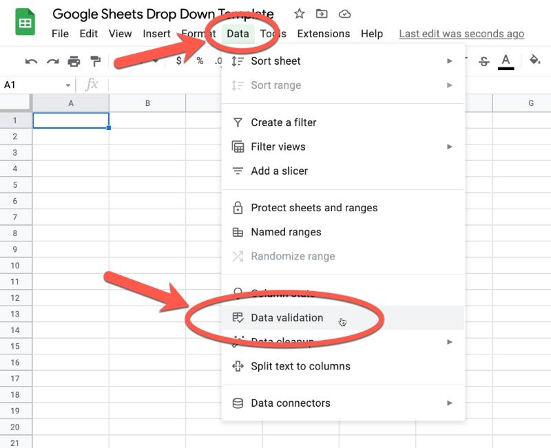
Note: you can also add a data validation rule by right-clicking on the cell, then choose:
View more cell actions > Data validation
Step 2: Add Drop-Down Options
From the data validation rules menu, select +Add rule
Then, choose either Dropdown or Dropdown (from a range) under the Criteria selection.
Dropdown
The Dropdown setup is the simpler one. You simply enter the values as you want them to appear in your list.
Here is the default drop-down setup that shows Option 1 and Option 2.
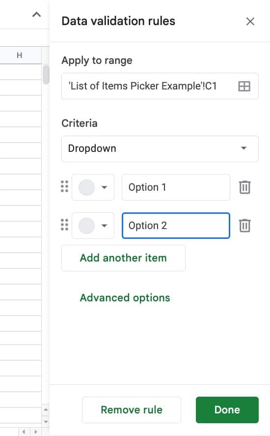
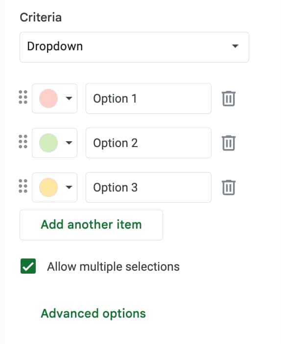
You can rename each option, change the color of each option, rearrange the order (by clicking and dragging on the dots to the left of each option), or add another item.
You can also enable multiple selections in drop downs, by toggling the checkbox under the options:
You’ll also notice the Advanced options button, which is discussed in detail below.
When you’re ready, click Done to add the drop-down menu to your cell.
Dropdown (from a range)
Typing a long list of items is impractical and error-prone, so if you have more than a handful of items, I recommend using the Dropdown (from a range) criteria option.
In this case, you create a list of all the possible items somewhere in your Google Sheet and link to that.
For example, suppose we want users to select which state they’re based in.
Leaving this as a free entry input cell would be a bad idea because we’ll get a huge number of variations (e.g. “CA”, “Cali”, “California”, etc.) which will all be interpreted differently by the Sheet.
Equally, typing all 50 states into the data validation as a list of items is inefficient.
A better option is to make a list of the items in your Sheet and link to that, as shown in this image:
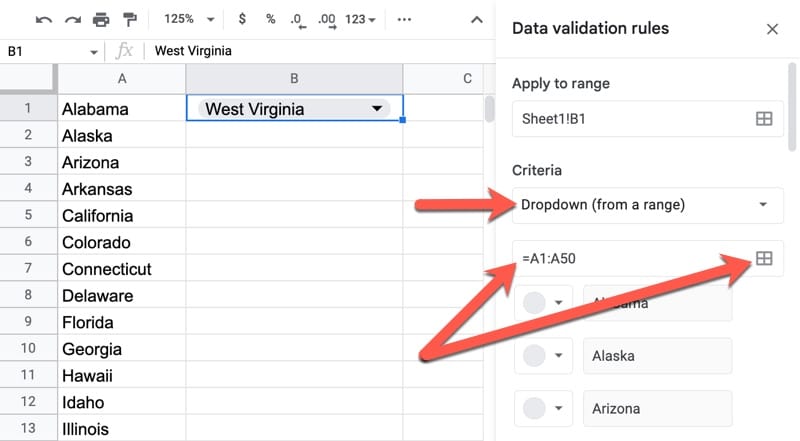
You can either enter the range as a formula, e.g.
=A1:A50Or click the grid in the input box, which opens a second popup that lets you select the range with your mouse:
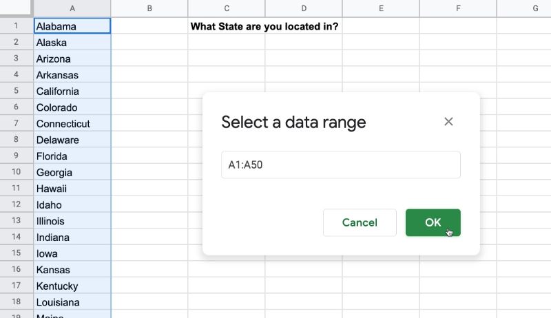
Click OK once you’ve selected the range for the drop-down items.
Then click Done to add the drop-down menu to your cell.
Step 3: Advanced Options
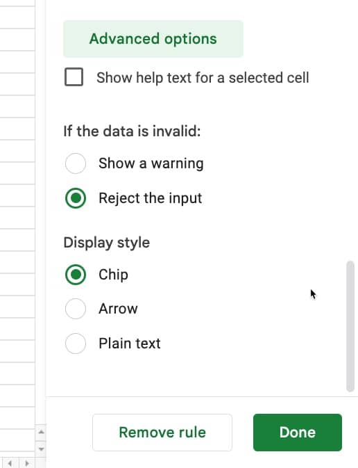
The Advanced options button lets you customize the drop-down menu:
Specifically:
• Show help text for a selected cell lets you specify a note to help users when selecting from the drop-down.
• The If the data is invalid option is useful to warn users if the value they are trying to enter differs from the options in the drop-down menu.
For example, if your drop-down selection is Blue or Red, but a user types Green into that cell, then you can either show a warning message or outright reject the input.
• The Display style option determines how the drop-down is presented in your Sheet.
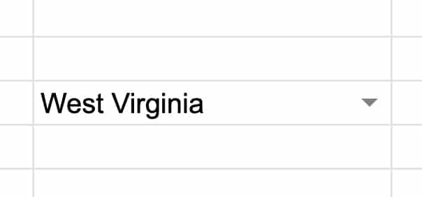
The Chip option looks like this:

The Arrow option like this:
And the Plain text like this:
To access the menu with the Plain text, double-click on the cell.
Note: the colors of the drop-down cells come from the colors specified in the list of items, above the Advanced options section.
Step 4: Reuse
Thankfully you don’t have to re-enter the list for each new cell you want to use the drop-down in.
Simply copy the cell with the drop-down and paste it elsewhere. The drop-down menu will be available in that cell too.
Drop Down Template
Click here to open a view-only copy >>
Feel free to make a copy: File > Make a copy…
If you can’t access the template, it might be because of your organization’s Google Workspace settings. If you right-click the link and open it in an Incognito window you’ll be able to see it.
You can also read about drop downs in the Google Documentation.
Google Sheets Drop Down Examples
Better User Input With Drop-Down Lists
The classic use case for a drop-down list in Google Sheets is to create a pre-defined set of inputs that users simply select when they’re entering data.
This is known as data validation (hence why we build drop-downs through the data validation menu).
Consider this example: suppose you’re collecting data about student grades and you require teachers to enter what grade a student belongs to.
You’ll get a mix of answers: 5, 5th, 5th Grade, Fifth, Fifth Grade, etc.
This causes problems because Google Sheets treats all of these as different answers in formulas or pivot tables. Before you can use this data, you’ll have to standardize it so that they’re all recorded as e.g. “5th Grade”.
But if you set your column up with a drop-down input, with choices “1st Grade”, “2nd Grade”, “3rd Grade”, etc., then you’ll avoid this problem altogether and save yourself tons of time.
Here’s how that column would look, using the Arrow display style:
I also use drop-down lists in the Google Sheet my wife and I use to track our spending habits.
The drop-down is a list of transaction categories (e.g. Food, Gas, Insurance, Health, Gifts, etc.). You can imagine how much easier, quicker, and more reliable this system is versus having a freeform input field.
Dynamic Charts Using Drop-Down Menus In Google Sheets
Along with checkboxes and slicers, it’s a great way to add interactivity to your Sheets and let your users control the data.
Dynamic charts really enhance reports and dashboards, allowing for more information to be conveyed in the same amount of screen space.
You can create dynamic charts by combining a drop-down menu in Google Sheets with lookup formulas. When the Google Sheets drop-down value changes, the formulas update their values, and then the chart updates in turn too.
See this article on dynamic charts in Google Sheets.
Dashboards Using Drop-Down List In Google Sheets
Consider this example of a dynamic dashboard, which shows a drop down list in Google Sheets to control the data displayed in the chart:
It lets users explore the data on their own terms and change what they’re seeing.
As you can see, the user is shown a choice of options that control some action downstream.
In this case, the drop-down list lets the user select a parameter (sales channel or time period) and updates the charts based on this choice automatically.
It makes the dashboard really pop! It lets the viewer explore the data in their own way.
Advanced Dependent Drop-Down Menus
It’s possible to combine two (or more) drop-downs that are conditional upon each other. I.e. the selection in the first drop down determines what items are shown in the second drop down.
Learn how to create dependent drop downs on Day 4 of my free course Advanced Formulas 30 Day Challenge.
Hi Ben…
I really enjoyed your tips that you shared in this website and Twitter. I just made multiple row and dependent drop down list for 2 columns (or even more). I want you to check if you can make it more simple. Thank you in advanced.
https://docs.google.com/spreadsheets/d/1c52F9eKOsyMY32Fty0QtiRZmPQM4gPeD0qZwjjma6w4/edit?usp=sharing
Ben, do you know if there are any plans to add a multi-select funcionatilty to dropdowns? That would certainly be a game-changer for sheets functionality…
It would be indeed! That would be lovely to have 🙂
But, sadly, I don’t know of any plans to add this functionality. You can always use slicers, which do allow multi-select: https://www.benlcollins.com/spreadsheets/slicers-in-google-sheets/
Multi-select using Slicers is a good call, but because they are designed to control filters it’s tricky to use the ‘result’ of a slicer in a formula because they sit ‘on top’ of the sheet rather than within a cell like a data validation drop-down. Here’s a hacky approach to extract the output of a slicer without resorting to scripting:
1. Enter the title your want for your slicer in A1
2. Enter the source list of items for the slicer in A2:Ax
3. Set up a slicer using A1:Ax as the source range, and move the slicer control into another sheet
4. In the same sheet as the slicer control, in any cell enter the formula =filter(range,map(range,lambda(x,subtotal(103,x)))) – this will output an array corresponding to the slicer output.
5. Deselect some of the items in the slicer, and watch what happens to the output of the formula… we are using the fact that the slicer filters the source list, but SUBTOTAL(103 within a MAP/BYROW generates a 1 or 0 for each row in the source list depending on if it is being filtered out or not, and this can be used as the input to a FILTER function elsewhere to return the selected items.
N.B. 1 – you need to keep the ‘Apply to Pivot Tables’ option in the Slicer settings enabled, otherwise the slicer output doesn’t update each time you make a change (not sure why)
N.B. 2 – If you want to use multiple slicers the source ranges musn’t overlap horizontally as SUBTOTAL(103 can only detect filtered rows, not individual cells. But stacking them vertically in a single column is fine.
N.B. 3 – For readability you could consider making the formula above into a named function (e.g. SLICER_OUTPUT(range), for instance)
N.B. 4 – I think there is an even more hacky way of doing multi-select using normal data validation drop downs with filtering and concatenation, but the Slicer approach is more elegant.
Hi Ben,
Thanks for the update on this. Does you 30 day course show you how to link a dynamic dropdown list items, t
another range, which displays the resultant data when making a selection from the dynamic dropdown list. Eg dynamic dropdown list selections are in cells b1;b20, and a imported range table a30;$z. How do link the the dropdown selection item to filter the data in range a30:$z.
I’m not sure if this method meets your need, but it does allow you to place the dynamic options on another sheet and doesn’t require any script. Just import this named function. There are three different examples included in the spreadsheet.
https://docs.google.com/spreadsheets/d/1SainCvS1RI_-UhIxXkT3KgFVcl0lmZM8rHsw_mBqPTA/edit?usp=sharing
The new Data Validation is making it difficult for Google Sheets Mathematicians.
When using Data Validation, I was able to use comma as separator for each data from the list.
Now, I have to manually enter each data or assign a range for my data.
And the data range can be re-used in other data validation formula, thus creating confusion.
I hope they will restore the original Data Validation, so I can continue creating video solutions for Taylor and Maclaurin SERIESSUM in Google Sheets.
I really like the chip view, especially the ability to differentiate options by color.
One note is that they are unfortunately vulnerable to being deleted accidently (like check boxes). If you have a value in a chip and press delete then it clears the value but leaves the chip. However, if you click delete on a chip when nothing is selected, then it removes the chip and validation altogether.
This won’t be an issue for tools that the creator is using regularly (and can fix if deleted). But if developing a tool that you will be sending out into the world or used by several less sheets savy users, it is worth thinking about if a user might accidently click delete and remove the dropdown. This isn’t an issue with arrow or text validation options.
Im hoping to find help with creating a very complex formula. I’m new to Google Spreadsheets, and attempting to create a comprehensive ROI/TC0 calculator that will be shared with internally and with our clients. I’m using 3 sheets inside the same document,
Sheet one will be presented to clients this is the ROI forecast. The data automatically populated will need to be from the second sheet. 2. The second sheet is for collecting the inputs and calculating our prices. 3. The third sheet is our Pricing matrix.
The second sheet, has 3 dropdown. One in each cell, which are critical to accurately price our solutions.
Dropdown A is the # of employees the organizations has, which I have very specific numbers. 100,000, 200,000, 250,000, and then it goes to 3M.
Dropdown B is the type of bundle of products the customer chooses. There’s 3 options that they can choose from.
Drop down C is the contract length term – 1 year, 2 , 3 year.
In my pricing matrix sheet I have this structured as, column A is # of employees, which are the same numbers from the dropdown option in the different sheet inputs tab. The only difference is, in the pricing matrix, it’s not a drop down, and each number is listed 3x since column B is the length, year 1 and 2 and 3, and then repeated . The rest of the columns are the bundle prices.
Not sure where to start, and what’s important, and how to do so it or even figure out how. I’ve tried lots of complex formulas but it’s not working. Any insights you can provide would be greatly appreciated.
Hi Ben. Thanks for this great post. I’ve got a question. I have a long list to cycle through and I’ve noticed that selecting an item moves it to the top of the list (temporarily) until another item is selected. Is there any way to have items stay put in the list as you select them? I’m finding it too easy to lose my place. I’m envisioning just being able to scroll down the list using arrow keys. Is anything like this possible? Thanks so much. Rich
Hi Ben, great info. Thanks for sharing. I finally understand more about sheets. I wanted to ask you about filters, for some reason, they aren’t working when applied. I can see my first row with the filter icon on each cell but it won’t show the values in the column, just shows up blank. Can you help me out here, please?