Coming hot on the heels of last year’s batch of new lambda functions, Google recently announced another group of new analytical functions for Sheets.
Included in this new batch are the long-awaited LET function, 8 new array manipulation functions, a new statistical function, and a new datetime function.
Let’s begin with a look at the new array functions. The LET function is at the end of the post.
- TOROW Function
- TOCOL Function
- CHOOSEROWS Function
- CHOOSECOLS Function
- WRAPROWS Function
- WRAPCOLS Function
- VSTACK Function
- HSTACK Function
- MARGINOFERROR Function
- EPOCHTODATE Function
- LET Function
New Array Manipulation Functions
Although there are eight new array manipulation functions, you can think of them as four pairs of horizontal/vertical array functions.
Although most of this behavior was already possible with existing functions, these new functions simplify the syntax and are therefore a welcome upgrade. They also maintain function parity with Excel, which will help folks coming from that world.
TOROW Function
TOROW transforms a range into a single row.
This formula turns the input array in A1:C2 into a single row:
=TOROW(A1:C2)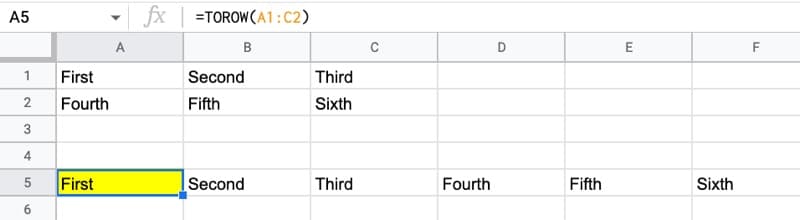
It has optional arguments that determine how to handle blank cells or error values, and also whether to scan down columns or across rows when scanning the input range.
More information in the Google Documentation.
TOCOL Function
The TOCOL function transforms a range into a single column. It behaves in the same way as the FLATTEN function.
This formula in cell A5 transposes each row into a column format and puts them one atop another:
=TOCOL(A1:C2)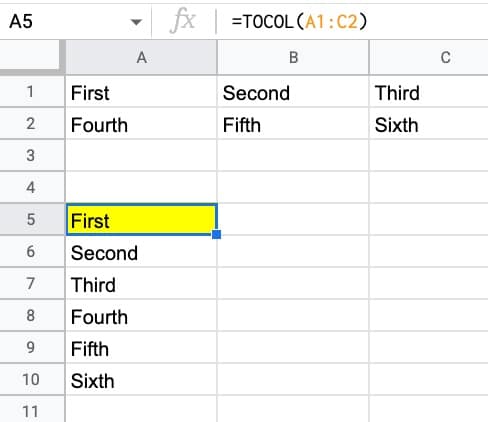
Like the TOROW function, it has optional arguments that determine how to handle blank cells or error values, and also whether to scan down columns or across rows when scanning the input range.
More information in the Google Documentation.
CHOOSEROWS Function
Given a range of data, the CHOOSEROWS function lets you select rows by row number.
For example, this formula selects the first, second, and fourth rows:
=CHOOSEROWS(A1:C5,1,2,4)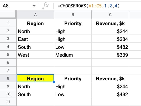
This can also be achieved, of course, by the FILTER function or the QUERY function. However, this new function is a nice, lightweight alternative for when you know the row numbers and don’t need to perform a conditional test on each row.
More information in the Google Documentation.
CHOOSECOLS Function
CHOOSECOLS is a welcome addition to the function family.
It lets you select specific columns from a range, which previously required a QUERY function and was more awkward because you use letter references for the columns.
This example selects the first and third columns from the input range:
=CHOOSECOLS(A1:C5,1,3)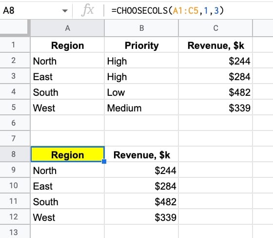
More information in the Google Documentation.
WRAPROWS Function
WRAPROWS takes a 1-dimensional range (a row or a column) and turns it into a 2-dimensional range by wrapping the rows.
It takes three arguments: 1) an input range, 2) a wrap count, which is the maximum number of elements in the new rows, and 3) a pad value, to fill in any extra cells.
In this example, the formula wraps the first row into multiple rows with a max of two elements on each row. Notice the second comma in the formula. This sets the pad value to blank, which means cell B8 is blank.
=WRAPROWS(A1:I1,2,)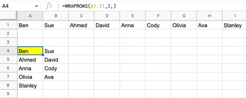
More information in the Google Documentation.
WRAPCOLS Function
WRAPCOLS takes a 1-dimensional range (a row or a column) and turns it into a 2-dimensional range by wrapping the columns.
It takes three arguments: 1) an input range, 2) a wrap count, which is the maximum number of elements in the new columns, and 3) a pad value, to fill in any extra cells.
In this example, the formula wraps the first row into multiple columns with a max of two elements down each column. Notice the second comma in the formula. This sets the pad value to blank, which means cell E4 is blank.
=WRAPCOLS(A1:I1,2,)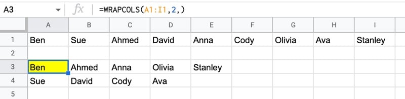
More information in the Google Documentation.
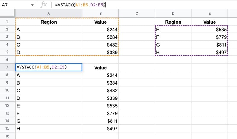
VSTACK Function
The VSTACK function stacks ranges of data vertically.
For example, you could VSTACK to easily combine two (or more) datasets:
=VSTACK(A1:B5,D2:E5)It takes the data in the range A1:B5 (which includes a header row) and appends the data from D2:E5 underneath, so you have it all in a single table:
More information in the Google Documentation.
HSTACK Function
HSTACK combines data ranges horizontally.
For example, this formula in A14 combines three data ranges horizontally:
=HSTACK(A1:A5,C3:C7,A7:A11)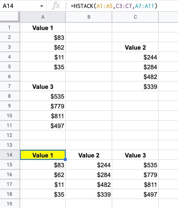
More information in the Google Documentation.
Margin Of Error Function
The MARGINOFERROR function calculates the margin of error for a range of values for a given confidence level.
It takes two arguments: 1) the range of values, and 2) the confidence level.
Let’s use this dataset as an example:
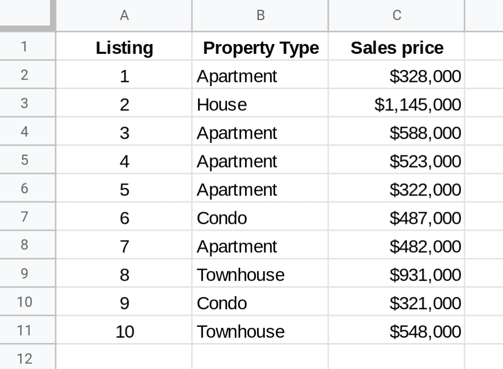
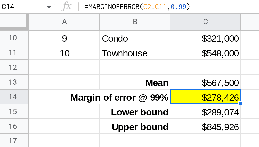
The MARGINOFERROR function is:
=MARGINOFERROR(C2:C11,0.99)which calculates the margin of error at a confidence level of 99%:
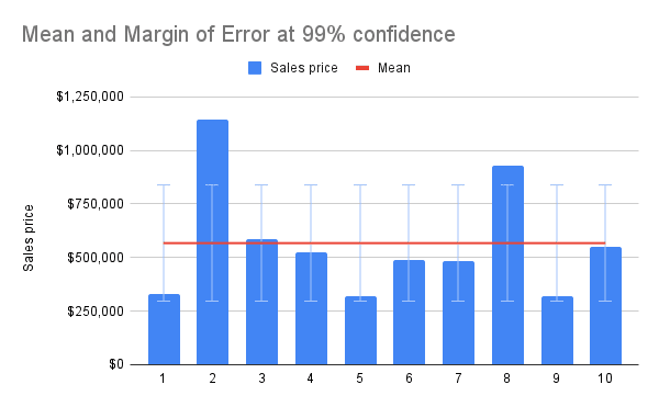
This is perhaps easier to understand on a chart, showing the margin of error bars (1 standard deviation) and the mean value (red line):
More information in the Google Documentation.
Epoch To Date Function
EPOCHTODATE converts a Unix epoch timestamp to a regular datetime (in Univerasal Coordinated Timezone, UTC).
It takes two arguments: 1) the Unix epoch timestamp, and 2) an optional unit argument.
A Unix timestamp looks like this:
1676300687
The EPOCHTODATE Function takes this as an input (e.g. the Unix timestamp is in cell A1 in this example):
=EPOCHTODATE(A1)
The output of the function is:
2/13/2023 15:04:47
More information in the Google Documentation.
LET Function
The LET function lets you use defined named variables in your formulas. It’s a powerful technique that reduces duplicate expressions in your formulas.
LET Example 1
Consider this LET example, which categorizes the total sales using an IFS function.
The LET function allows us to define a “sales” variable that references the SUM of sales in column C. We can reuse the variable “sales” anywhere else in this formula:
=LET( sales , SUM(C2:C11) , IFS( sales>6000000 , "Exceed target" , sales>5000000 , "On target" , sales>4000000 , "Below target" ))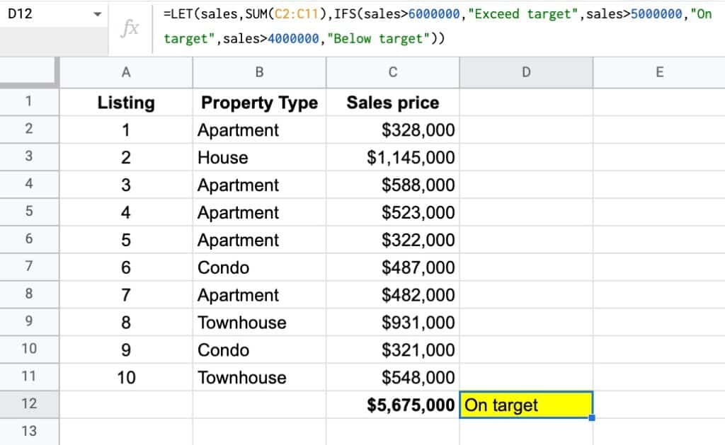
Without LET, the formula repeats the SUM expression repeatedly, which makes changing this formula more difficult:
=IFS( SUM(C2:C11)>6000000 , "Exceed target" , SUM(C2:C11)>5000000 , "On target" , SUM(C2:C11)>4000000 , "Below target")LET Example 2
This formula — using LET, SEQUENCE, and FILTER — will get all the weekdays (Monday – Friday) for the year ahead, starting from today:
=LET( dates , SEQUENCE(365,1,TODAY(),1) , FILTER( dates , WEEKDAY(dates,2)<6 ))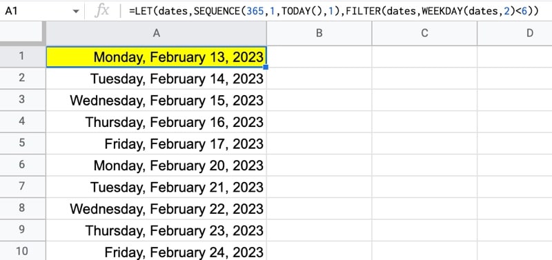
By using LET, you can avoid repeating the SEQUENCE expression.
More information in the Google Documentation.
Tocol and Torow will be useful Monday morning. Thanks for the good summary, Ben!
You’re welcome. Cheers, Per! I agree that these new functions will be very handy.
Thanks for your sharing. Interesting new functions.
A few days ago I had used choosecols function in my reports, but this morning the function result show “Unknown function: ‘CHOOSECOLS'”.
In this moment, I found function list when type choose, only display 1 function (CHOOSE).
They’re rolling out over a period of weeks, so you should get them soon…
All 11 of these functions were actually supposed to be rolled out by February 15th, but Google have temporarily pulled all eight of the new array manipulation functions because they were causing sheets to crash and lose data in some contexts…
Yes, they are currently unavailable (2/23/23), which is unfortunate!
Yeah, as of today the only ones working for me are:
MARGINOFERROR()
EPOCHTODATE()
LET()
Great content again, Ben. Thanks for the overview.
I was wondering what the usecase of VSTACK/HSTACK was over ={…}. In the examples in you article both could be used. VSTACK/HSTACK seems to be able to handle different size of row/columns, where curly brackets is very strict. Also seems to have more options for to giving/handling errors in cases where the array sizes do not match. Good improvement!
Hi Frank – I agree. I think the VSTACK/HSTACK will be more flexible and easier to use than the older array literals {…} that few people are even aware of.
Cheers,
Ben
Do we have any way of knowing if the performance of VSTACK and HSTACK versus {} arrays will be the same? I’m worried that while more convenient, in complex formulas it will be slow enough to be noticeable.
Great question… don’t know the answer yet, but it would be worth some research.
The only case where I found VSTACK better than {;} is when you pass arrays of different width to vstack. Example:
=VSTACK(A1:C1,B2,C2,A3,C3)
will trigger a #N/A error in the 3rd cell of the second output row that you can nix, by encapsulating vstack in an IFERROR, as in:
=IFERROR(VSTACK(A1:C1,B2,C2,A3,C3),”value for missing cells”)
You cannot do that with curly braces.
Are there other interesting cases for VSTACK/HSTACK ?
Elaborating on your point Jean-Rene, the most interesting use-case for me is when getting data from multiple sources (multiple sheets with the same output format) where a single source might be empty (no output). With the {} you’d get an error because that array is empty, with vstack you can catch the error and still get a result from the other output tables.
Great summary. I always appreciate how your posts keep me up-to-date on what Google’s releasing.
You’re welcome!
FYI Ben, a little mistake I think: it is the new TOCOL function that is the same as FLATTEN, not VSTACK as you wrote above. Flatten always returns a single column.
Good spot. Thank you! Fixed now.
How to create array to sum considering column & row headers
https://support.google.com/docs/thread/259751759?hl=en
So happy to have this in our very own Google sheet! These functions are all game changer…
This is great, thanks so much!
LET function is really powerful. Thank you for sharing!
Something weird is happening… I have tried all these functions in a new blank sheet, and they worked. Then I am using them in another sheet (that was created before this update) but getting “Unknown function” error for all the functions, excel LET and EPOCHTODATE. Same account and same PC. That seems, those functions don’t work within old sheets. Hope that will get fixed soon.
Oops – sent this as an email before scrolling down and seeing the comments section.
Hi Ben
Yours is the best website I have found for tips on Google sheets. Love it! Keep up the great work.
A suggestion on your excellent article on VStack . . .
It would help if it addressed this situation:
Our ranges to be stacked will continue to grow as we add data. One might be 50 rows long today and grow to 60 rows tomorrow and 90 rows next week. If we choose one or more ranges that go beyond the populated range to accommodate future growth–or even to the bottom of the page, such as =vstack(A4:D,G4:J55), then the stacked range will include all the empty rows of that range.
Perhaps there is a solution for that so we only get populated rows in the output?
Thank you, and keep up the great work!
Learned a lot of new functions. Will they work in Microsft Excel because 50% of my work is offline. Btw, thank you so much for the teaching.
The documentation doesn’t relay this but the real beauty of the hstack and vstack operations is that you can combine arrays that aren’t necessarily the same aspect ratio (sometimes called jagged arrays or ragged arrays). With the vstack and hstack you just get the #N/A in the cells where there’s a non-matching value for that column / row. This is very different from other array operations (such as use of {} together with “;” and ‘,’); those just return an error (mismatched row size, mismatched column size) and no part of the joined array. These new formulas make it much easier to debug because you can see what is mismatched, and sometimes you just don’t need them to match anyway.
One use for the LET function could also be for “documentation/readability”.
i.e. “sales>5000000” is easier to understand than “SUM(C2:C11)>5000000”.
I could see myself using it just for this purpose alone, I have sometimes used “+ N(‘This arrayformula does …’)” just to remind me “how this works” 6 months from now.
Great idea for comments
It works really well for this. It’s basically named ranges, but scoped locally inside your function.
Really useful insights on the new analytical functions! Can’t wait to try them out in my own spreadsheets—thanks for sharing!
I have been using the LET() function for documentation for some time now. I add a variable “vDoc” at the top and assign it a string. Then I ignore that variable in my formula. e.g.
=LET(
vDoc, “This adds two numbers then divides by
two to get the average of the two numbers.”,
vNum1, A1,
vNum2, B1,
(vNum1 + vNum2) / 2
)
I used to put that documentation in a cell “note” but I don’t like cluttering up my screen with those pop-up “note” bubbles. I also find it easier to keep that documentation current when it’s embedded in the formula. Last of all, I don’t have to take the extra steps to delete the “note” if I delete the formula.
Of course, this example formula isn’t anywhere near needing documentation but I have found it invaluable for the really complex formulae where the use of the variables saves making the same calculation multiple times within the same formula.
Yes! I do this too and it’s the best way to add comments to formulas in Sheets presently. Thanks for sharing, Chris!
Cheers,
Ben
Ben,
Thank YOU for all you do. I’m sure you’ve been a great help to many spreadsheet users out there. Keep up the good work!
SINCERELY,
Chris
You’re welcome! Thanks, Chris.