IFS Function in Google Sheets

The IFS function in Google Sheets is used to test multiple conditions and outputs a value specified by the first test that evaluates to true.

It’s akin to a nested IF formula, although it’s not exactly the same. However, if you find yourself creating a nested IF formula then it’s probably easier to use this IFS function.

Example IFS Function in Google Sheets

Suppose you have a set of student exam scores and you want to assign different grades to the students:

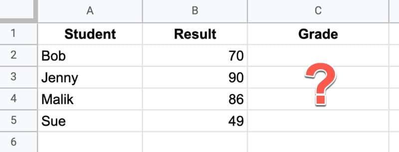
In this scenario, you want to put students into three groups: i) those who score below 50 failed the exam, ii) those with scores between 50 and 79 passed the exam, and iii) students who scored 80 or above passed with distinction.

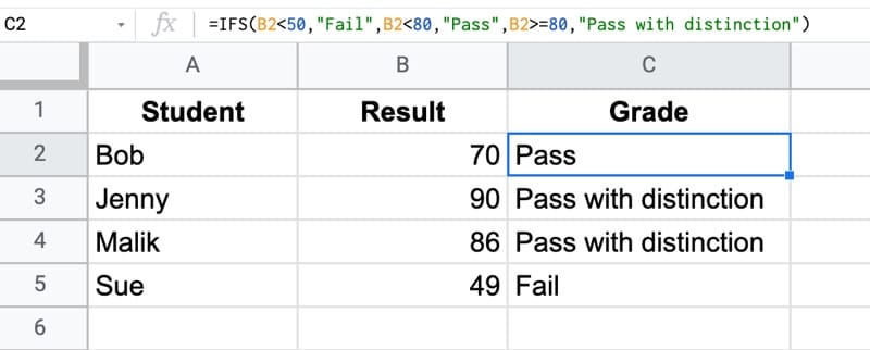
The IFS Function to do this is:

The IFS function consists of pairs of arguments: a condition to test and a value.

If the conditional test is true, the value is displayed and the function stops. If not, and the test is false, the function tries the next test/value pair.

Consider row 2 of the example above, where Bob has a score of 70 in cell B2.

The first logical test and value pair is:

The function takes the value of 70 in cell B2 and compares it to the value of 50 to see if it’s less. This is false, so the “Fail” output is not displayed.

Instead, the IFS function in Google Sheets moves to the second logical test and value pair:

This time the logical test – is 70 less than 80? – evaluates to true, so the function displays “Pass”.

The IFS formula never reaches the third test/value pair.

The result of the IFS function in Google Sheets is an output that classifies the students:

You could modify this IFS formula to assign grades “A”, “B”, “C” etc. instead, based on bands.

Note, it can also be done with a nested IF function. This gives the same result as the IFS function, but is more complex to understand:

IFS Function in Google Sheets: Syntax

It takes a minimum of two arguments: a condition & a value.

This is a logical test that evaluates to a TRUE or FALSE value. For example A1 > 10

If condition1 is TRUE, then the IFS function will output this value.

These are optional pairs of logical tests and values. If condition 1 is FALSE, the IFS moves on to test condition 2, then 3, then 4 etc.

IFS Function Notes

• The conditions and values always come in a pair, so the IFS always has an even number of arugments.
• The function reads the test/value pairs from left to right. It always starts with the leftmost argument as the first logical test.
• There is no default value to display should all the conditions fail. The IFS function will then output an #N/A! error.
• However, you can create a default fallback value by adding a penultimate argument TRUE (the logical test) and some value (the fallback value). This is illustrated in the bank account example below.

IFS function template

Click here to open a view-only copy >>

Feel free to make a copy: File > Make a copy…

If you can’t access the template, it might be because of your organization’s Google Workspace settings. If you click the link and open it in an Incognito window you’ll be able to see it.

You can also read about it in the Google documentation.

IFS Function Account Balance Example

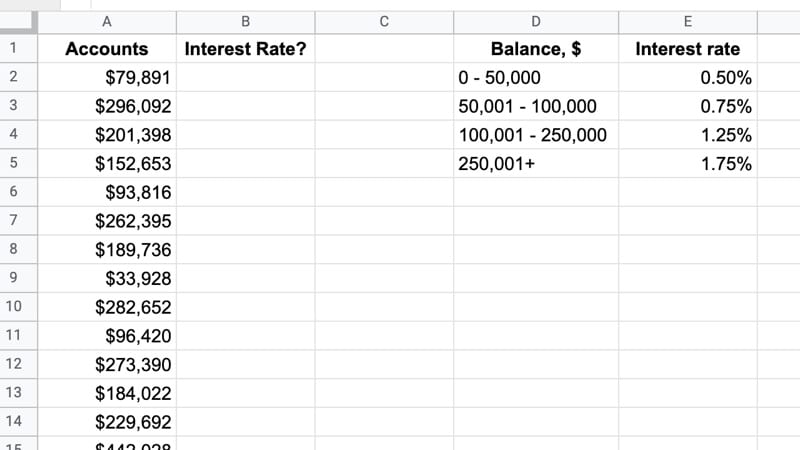
Suppose you have a list of corporate bank balances and a table of interest rates, and you want to add the correct rate against the account balance so you can calculate the interest.

One way to do this is to use this IFS function in cell B2:

The first test compares the value in cell A2 to see if it’s less than $50,001, which means the account balance is in the $0 – $50,000 tier, so the formula returns a value of 0.5%.

If this first test fails, it tries the second logical test. If that fails, it tries the third logical test, etc.

As it’s written above, the interest rates are hardcoded in the formula, which is generally bad practice (because it’s hard to make changes and easy to make mistakes).

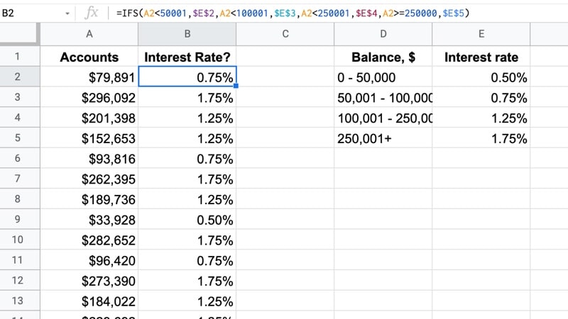
A better solution is to link the output values to the interest rate table, as shown in this version of the formula:

(Exercise for readers: take this a step further and link the bounds (50001, 100001 etc.) to the interest rate table instead of hard coding them.)

The output looks like this:

Note: The final logical test can be replaced with the word TRUE, as the catch-all when none of the other conditions are met:

Alternative Solution

Note that this account example can also be solved with the VLOOKUP function using a TRUE value as the final argument.

This account example is covered in Day 6 of my free Advanced Formulas 30 Day Challenge course.

You might also consider using the SWITCH function, which works for exact matches.

Advanced IFS Function in Google Sheets

This is somewhat contrived but will give you an idea of what’s possible with the IFS function.

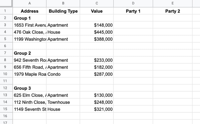
In this scenario, imagine that two parties of buyers have viewed some properties.

The agent wants to record each party’s preferences. He remembers:

“Party 1 liked apartments under $200k”

“Party 2 liked houses or townhouses”

There are various ways you could solve this, including simply recording the preferences manually in a Sheet, but let’s see an IFS formula that does it automatically.

Here’s the data table:

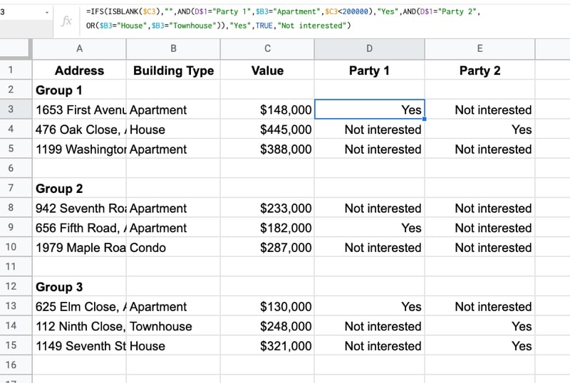
And here’s the formula in cell D2 that can be dragged down the column and across the row to fill in the peferences:

The test/value pairs are grouped as follows:

Test #	Test	In Formula	Output
1	Is cell C3 blank?	ISBLANK($C3)	""
2	Is it party 1 and Apartment and less than $200k?	AND(D$1 = "Party 1",$B3 = "Apartment",$C3 < 200000)	Yes
3	Is it party 2 and house or townhouse?	AND(D$1 = "Party 2",OR($B3 = "House",$B3 = "Townhouse"))	Yes
4	Catch all when conditions 1 – 3 not true	TRUE	Not interested

You’ll notice that test/value pairs 2 and 3 show how to use a nested AND function and a nested OR function to combine conditions.

The output of this formula is: