The VLOOKUP function in Google Sheets is a vertical lookup function. You use it to search for an item in a column and return data from that row if a match is found.
In the following example, we use a VLOOKUP formula to search for “Charles Dickens” in column 1. When we find it, the formula returns the value from the 4th column of the lookup table to give a result of $299.
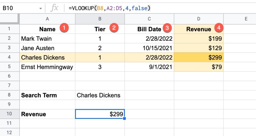
In this example, the VLOOKUP function is:
=VLOOKUP(B8,A2:D5,4,false)Let’s break this formula down:
B8 is the search term: “Charles Dickens”
The VLOOKUP looks down the first column of the lookup table: A2:D5
If it finds the search term, it then looks across that row to the column indicated by the Index number: 4
It then returns the value from column 4 as the answer, which is $299 in this example.
The final argument is false, meaning this is an exact match.
VLOOKUP can also handle approximate matching as well as wildcard searches. These more advanced use cases are explored further below.
VLOOKUP Function Syntax
Here is the VLOOKUP syntax:
=VLOOKUP(search_key, range, index, [is_sorted])The name VLOOKUP stands for Vertical Lookup. It gets this name because it searches for a value up and down a column, i.e. vertically, rather than horizontally. The horizontal lookup, which is used much less frequently, is called the HLOOKUP.
search_key
The search_key is the item from the original table that you want to search for in the lookup table.
range
The second argument, range, is the lookup table, i.e. the table we’re going to search in.
VLOOKUP always searches down the first column of this table.
index
If the search term is found, the value from a specific cell of that row is returned. The index value (the third argument) determines which column of the lookup table to use.
If the index number is greater than the number of columns in the lookup table (i.e. you’re asking the VLOOKUP formula to return values from column 4 of a lookup table that only has 3 columns), a #REF! error is returned.
is_sorted
The final argument takes a TRUE or FALSE value, sometimes written as 1 (TRUE) or 0 (FALSE).
FALSE means:
- It does exact matching
- It is not case senstive
- If there are multiple matches, the first match is found and the return content is taken from that row (i.e. if Ben Collins appears twice in the lookup table on row 5 and row 10, then information from row 5 is always returned)
- If no lookup value is found, VLOOKUP returns the #N/A error message
- The FALSE setting is used for 99% of VLOOKUP cases
Whereas TRUE means:
- It finds the nearest match that is less than or equal to the search key
- This option is rarely used
VLOOKUP function template
Click here to open a view-only copy >>
Feel free to make a copy: File > Make a copy…
If you can’t access the template, it might be because of your organization’s Google Workspace settings. If you click the link and open in an Incognito window you’ll be able to see it.
VLOOKUP To Join Tables In Google Sheets
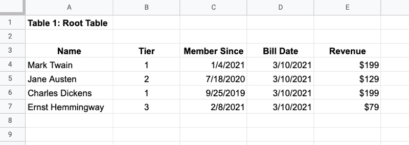
The VLOOKUP function in Google Sheets is typically used to bring data from one data table and add it into another.
Suppose we run a Saas startup for famous writers, who each pay a monthly fee to subscribe to our service:
In addition, we have a separate customer table that contains their location details:
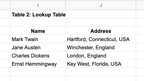
To truly understand our sales data, we want to combine these tables so we can see revenue by location.
We use this VLOOKUP function:
=VLOOKUP( A4,$I$3:$J$7,2,false)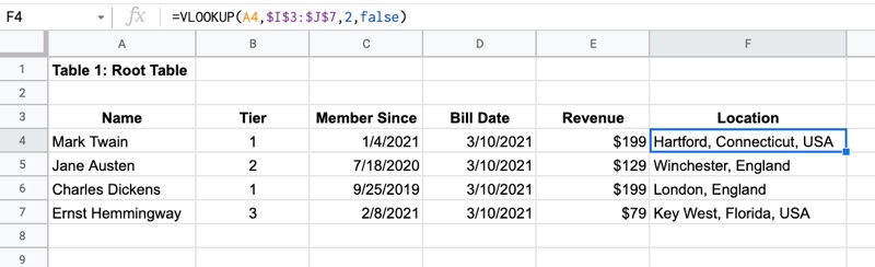
The $ signs around the table range reference make it an absolute reference, which locks the range reference in place.
This is often required for VLOOKUPs so that when you copy the formula, the lookup table does not change. Use the F4 key to quickly add or remove dollar signs.
Approximate matching using A VLOOKUP Formula with TRUE argument
This VLOOKUP lesson is from Day 6 of my free Advanced Formulas 30 Day Challenge course.
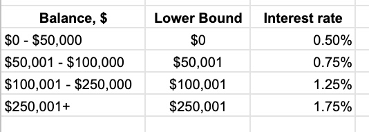
Suppose you know the interest rates at your bank:
And then you have a bunch of accounts for which you want to calculate the interest:
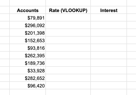
It would be tedious to manually lookup each account value in the interest table and determine the rate.
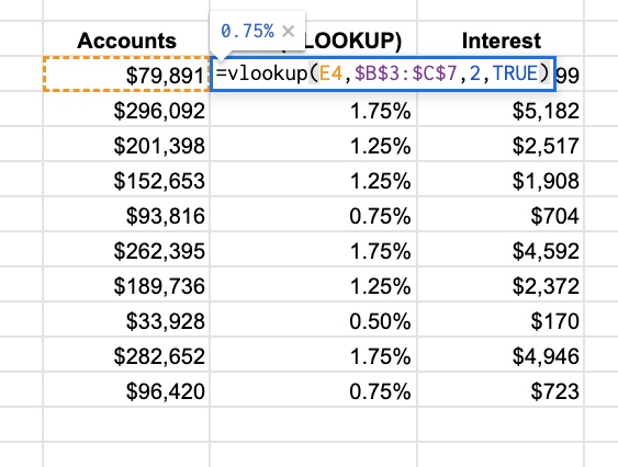
What you can do is use the VLOOKUP with the TRUE argument.
In this example, I have an ordered list of values in column B, from lowest to highest, that denote the different brackets for the interest rate bands.
When I lookup a value (e.g. $79,891) the VLOOKUP TRUE will search down column B until it reaches a number larger than the search value, then stop on that row before that larger value. In this example, it will stop at $50,001 because the next value, $100,001, is larger than the $79,891. So it returns an interest rate from the $50,001 row because that represents the $50,001 – $100,000 band that the interest rate is in.
It finds the nearest match that is less than or equal to the search key.
The result of the VLOOKUP is:
Using The VLOOKUP Function in Google Sheets To Compare Data Lists
Another common use case for VLOOKUP is to compare two lists of data, for example, names, and determine what the differences are.
You compare lists by looking for names from list 1 in list 2 and then vice versa, looking for names from list 2 in list 1.
The VLOOKUP formula might look like this:
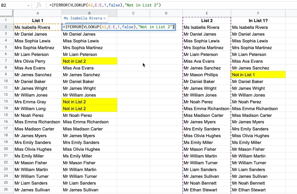
=IFERROR( VLOOKUP( A2 , E:E , 1 , false ) , "Not in List 2" )A few things to note about this formula:
- The lookup table is a single column E:E
- So the index must be 1
- With index 1, it returns the name if it’s found
- It uses the IFERROR function to display a custom error message when names are not found
Here is a list comparison example in practice (click to enlarge):
Advanced VLOOKUP Techniques
VLOOKUP In Google Sheets Using Wildcards For Partial Matches
How to use wildcard characters “*” to perform partial matches in Google Sheets.
How To VLOOKUP To The Left In Google Sheets?
Regular VLOOKUP formulas will only return values from columns to the right of the lookup column. However, there’s a technique using Array Literals that lets us return values from columns to the left of the lookup column.
Have Vlookup Return Multiple Columns in Google Sheets
Have you ever wanted to return more than a single column with VLOOKUP? Perhaps you want to combine two tables and bring all the data across. This tutorial will show you how to do that without requiring multiple VLOOKUP formulas.
VLOOKUP Multiple Criteria in Google Sheets
This tutorial shows you how to perform a VLOOKUP using multiple input criteria. For example, you can combine first name and last name inside the VLOOKUP to search against a full name column.
You can also read about it in the Google documentation.
Thank you so much for this guide and also for sharing the template so I can practice it.
I came here from https://twitter.com/glenngabe/status/1371433916289183746?s=20
Thank you! Glad to hear it’s been helpful.
Hi,
Is there any app script way of performing VLOOKUP?
Curious to know.
How we can find the value from different Google Sheet using vlookup formula
Can you use this to look in a row for condition 1, then look down in that collumn for condition 2 and if the second contion is true then show the value of cell a1 of that row. (and skip all rows that doesnt fit condition 2)