How To Use Google Sheets SUMIF Function

The SUMIF function in Google Sheets is used to sum across a range of cells based on a conditional test. The SUMIF function only adds values to the total when the condition is met.

Let’s see an example. Suppose we want to calculate the total order value for John only:

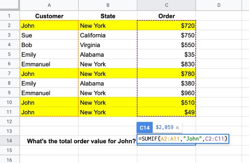
The SUMIF formula that calculates the total order value for John is:

which gives an answer of $2,059.

The formula tests column A for the value “John”, and, if it matches John, adds the value from column C to the total. I’ve highlighted the four rows in yellow that are included.

🔗 Get this example and others in the template at the bottom of this article.

SUMIF Function Syntax

It has two mandatory arguments and one optional argument.

range

The range is the data that you want to test with your criterion. If the third argument (sum_ragne) is omitted then this range will also be used for the sum.

criterion

The criterion is the test you want to apply. If you want to apply multiple tests to your sum, then you need to use the SUMIFS function.

[sum_range]

This is an optional argument that lets you specify a different range to use to calculate the sum total. It must be the same size as the test range.

SUMIF Function Notes

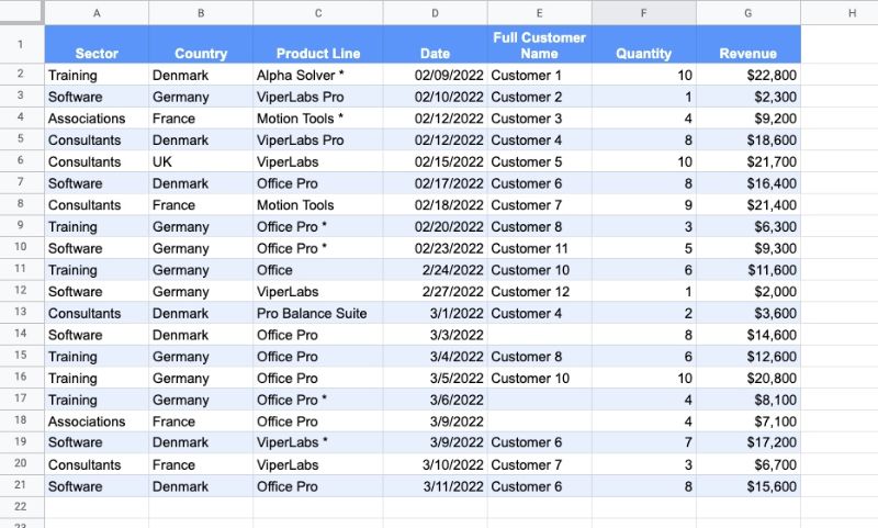
The following dataset (available in the template below) is used in all the examples that follow:

Text Criterion

Text criterion must be enclosed by quotes.

This formula calculates the total revenue for Germany:

Numeric Criterion

Exact matches with numeric values do not require quotes but logical tests do require quotes.

For example, this formula calculates the total revenue from orders that have exactly 10 items as the quantity:

However, if the criterion includes a logical test, then the formula requires double-quotes.

For example, this formula calculates the total revenue of orders where revenue > $20k:

Notice how this last SUMIF formula does not include the optional sum range. In this case, the conditional range to test is also the range used for the sum.

Conditional Tests

Logical operators are used to create conditional tests:

• > greater than
• >= greater than or equal to
• < less than
• <= less than or equal to
• = equal to
• <> not equal to

They must be enclosed with double-quotes.

This formula calculates the total revenue of orders with more than 5 items:

Case Insensitive

The SUMIF function is case insensitive, so “john”, “JOHN”, or “John” will all produce identical results.

SUMIF Function with Blanks and Non Blanks

To sum blank cells in a range, use empty double-quotes:

To sum non-blank cells in a range, use the not-equal logical operator “<>“:

Reference another cell

The test criterion for SUMIF function can be contained in a different cell (in this example G26) and referenced by the SUMIF formula:

If you want to use a logical operator, then it must still be enclosed in double-quotes. Use an ampersand to combine with the reference cell, e.g.

Using Wildcards with SUMIF

SUMIF Google Sheets supports three wildcards, *, ?, and ~.

The star * matches zero or more characters.

The question mark ? matches exactly one character.

The tilde ~ is an escape character that lets you search for a * or ?, instead of using them as wildcards.

Let’s see some examples:

Star Example

What’s the revenue from “Pro” products?

This formula finds everything containing “Pro”:

Question Mark Example

What’s the revenue from customers 10, 11, and 12 combined?

This can be achieved in two ways. Firstly, using a SUMIF for each of the customers and adding them together, like so:

Or, you can use a question mark as a placeholder to catch 10, 11, and 12 in one go, like this:

The question mark matches a single character, so only Customers 10, 11, and 12 will match. This is obviously specific to this dataset but illustrates how the question mark works.

Both of these formulas give the same answer of $43,700.

Tilde Example

The tilde escape character lets you search for a * or ? without the special meaning above being applied.

For example, to calculate the revenue of Office Pro products with a * next to their name in the table above, we use:

SUMIF Function Template

Click here to open a view-only copy >>

Feel free to make a copy: File > Make a copy…

If you can’t access the template, it might be because of your organization’s Google Workspace settings. If you right-click the link and open it in an Incognito window you’ll be able to see it.

The SUMIF function is also covered in Day 2 of my free Advanced Formulas 30 Day Challenge course.

SUMIF is part of the Math family of functions in Google Sheets. You can read about it in the Google Documentation.

See Also

For conditional counting, have a look at the COUNTIF function and COUNTIFS function. They work in the same way as SUMIF but count the values that match the criterion.