The Google Sheets SUMIFS function is used to sum ranges based on conditional tests. In other words, the SUMIFS in Google Sheets adds values to a total only when multiple conditions are met.
Suppose we want to calculate the total for Large products in New York:
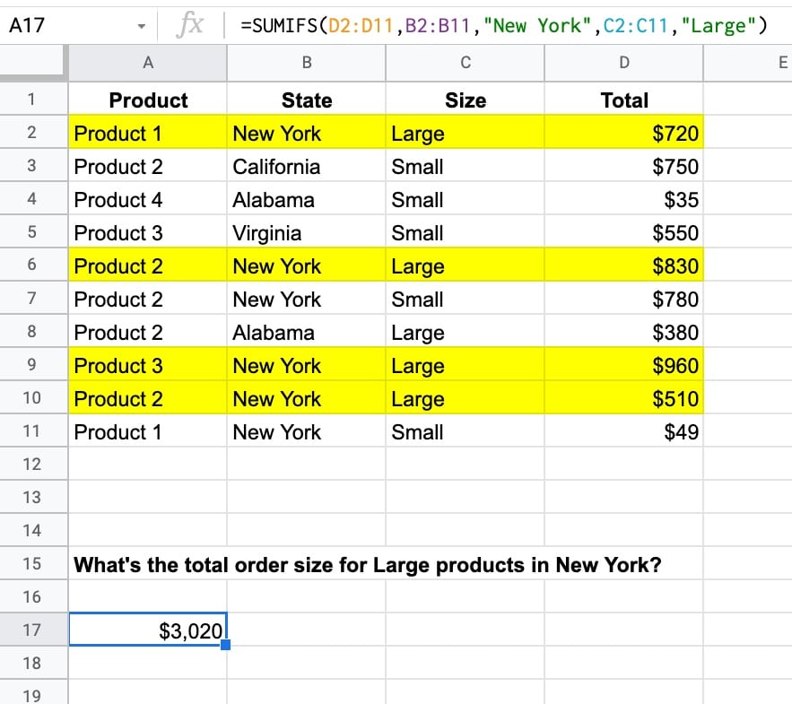
The SUMIFS function to calculate the total for two conditions, Large and New York, is:
=SUMIFS(D2:D11,B2:B11,"New York",C2:C11,"Large")which gives an answer of $3,020.
In this case, there are four rows, highlighted in yellow, that match the criteria of New York in column B and Large in column C.
The total values of these four rows are added together by the SUMIFS function, all the other rows are discarded.
🔗 Get this example and others in the template at the bottom of this article.
Google Sheets SUMIFS Function Syntax
=SUMIFS(sum_range, criteria_range1, criterion1, [criteria_range2, criterion2, ...])It takes a minimum of three arguments:
sum_range
This is the range to use to calculate the sum total.
criteria_range1
This range is the data that you want to test with your criterion. It must be the same size as the sum range (i.e. have the same number of rows).
criterion1
The criterion is the test you want to apply.
Although it works perfectly well with a single criterion, it’s more common to use the SUMIF function in this case. Just be aware that the order of the test range and the sum range are reversed in the SUMIF.
[criteria_range2, criterion2, ...]We can add optional pairs of range/tests to SUMIFS to test more conditions. Each range must match the size of the original sum range (i.e. have the same number of rows).
SUMIFS Function Notes
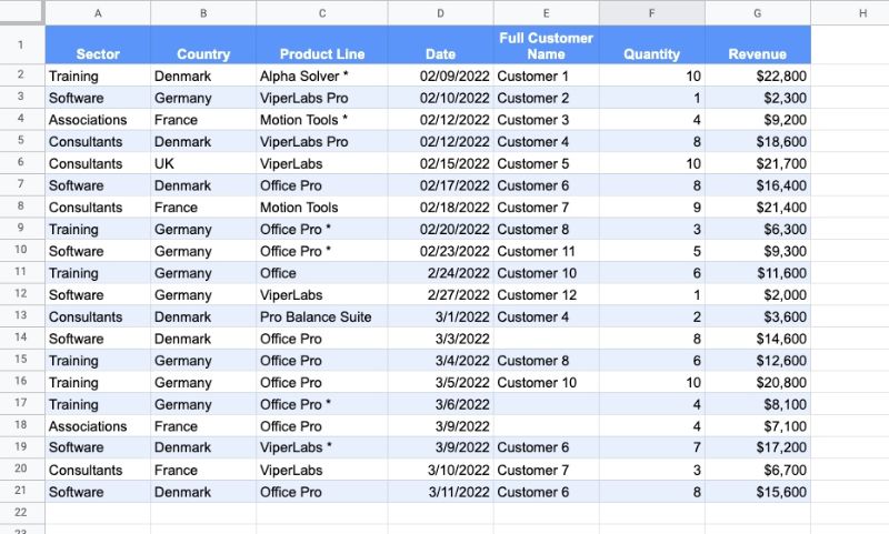
The following dataset (available in the template below) is used in all the examples that follow:
Text Criterion
Text criterion must be enclosed by quotes.
This formula calculates the total revenue for the Training sector in Denmark:
=SUMIFS(G2:G21,A2:A21,"Training",B2:B21,"Denmark")Numeric Criterion
Exact matches with numeric values do not require quotes but logical tests do require quotes.
For example, this formula calculates the total revenue from Consultant sector orders that have exactly 10 items as the quantity:
=SUMIFS(G2:G21,A2:A21,"Consultants",F2:F21,10)However, if the criterion includes a logical test, then the formula requires double-quotes.
For example, this formula calculates the total revenue of orders where revenue > $20k:
=SUMIFS(G2:G21,G2:G21,">20000")Notice how this last SUMIFS formula only has three arguments, i.e. one pair of test range + criterion.
In this case, a SUMIF would also work and is more succinct:
=SUMIF(G2:G21,">20000")Conditional Tests
Logical operators are used to create conditional tests:
- > greater than
- >= greater than or equal to
- < less than
- <= less than or equal to
- = equal to
- <> not equal to
They must be enclosed with double-quotes.
This formula calculates the total revenue for the Training sector and orders with more than 5 items:
=SUMIFS(G2:G21,A2:A21,"Training",F2:F21,">5")Case Insensitive
The SUMIFS function is case insensitive. For example, testing for “training”, “TRAINING”, or “Training” will all produce identical results.
SUMIFS Function with Blanks and Non Blanks
To sum blank cells in a range, use empty double-quotes.
For example, this formula tests for Software and blank customer names:
=SUMIFS(G2:G21,A2:A21,"Software",E2:E21,"")To sum non-blank cells in a range, use the not-equal logical operator “<>“.
Here, this formula tests for Germany and non-blank customer names:
=SUMIFS(G2:G21,B2:B21,"Germany",E2:E21,"<>")Reference another cell
The test criterion for SUMIFS function can be contained in a different cell and referenced by the SUMIFS formula:
=SUMIFS(G2:G21,A2:A21,G27,B2:B21,G28)If you want to use a logical operator, then it must still be enclosed in double-quotes. Use an ampersand to combine with the reference cell, e.g.
=SUMIFS(G2:G21,A2:A21,"Training",F2:F21,">"&J28)Using Wildcards with SUMIFS
SUMIFS Google Sheets supports three wildcards, *, ?, and ~.
The star * matches zero or more characters.
The question mark ? matches exactly one character.
The tilde ~ is an escape character that lets you search for a * or ?, instead of using them as wildcards.
Let’s see some examples:
Star Example
This formula calculates the revenue from “Pro” products from Denmark:
=SUMIFS(G2:G21,B2:B21,"Denmark",C2:C21,"*Pro*")It will include “Office Pro”, “Pro Balance Suite”, “ViperLabs Pro”, etc.
Question Mark Example
This formula calculates revenue from customers 10, 11 or 12 in Software sector:
=SUMIFS(G2:G21,A2:A21,"Software",E2:E21,"Customer 1?")Tilde Example
The tilde escape character lets you search for a * or ? without the special meaning above being applied.
For example, this formula calculates total revenue for Germany and starred products Office Pro *:
=SUMIFS(G2:G21,B2:B21,"Germany",C2:C21,"Office Pro ~*")Error Message
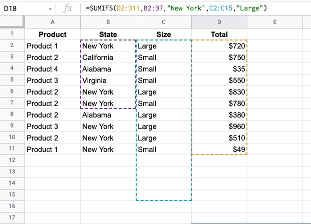
If your input ranges are different sizes then you’ll see a #VALUE! error, saying “Array arguments to SUMIFS are of different size.”.
which results in this error message:
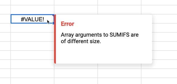
It’s easily fixed: simply change your ranges to be the same dimensions, i.e. all have the same number of rows.
SUMIFS Function Template
Click here to open a view-only copy >>
Feel free to make a copy: File > Make a copy…
If you can’t access the template, it might be because of your organization’s Google Workspace settings. If you right-click the link and open it in an Incognito window you’ll be able to see it.
The SUMIFS function is also covered in the Day 2 lesson of my free Advanced Formulas 30 Day Challenge course.
It’s part of the Math family of functions in Google Sheets, along with its siblings the SUMIF function (for a single criterion), the COUNTIF function (for counting with a single criterion), and the COUNTIFS function (for counting with multiple criteria).
You can also read about it in the Google Documentation.
I’m trying to set up a sheet to track expenses with month summary rows at the top.
A: Date
B: Expense description
C: amount
D: confirmation number
E: category
F: payment method
G: notes/comments
H and beyond are specific categories of expenses (e.g., Capital One, Rent, Phone, etc.) because we need to track totals of expenses in each of those categories.
E tells the sheet to put the amount (C) in which column (H and beyond) and uses an IF function. which is working properly.
Row 1 is header row
Rows 2+ are monthly summary rows (April 2022, May 2022, etc), grouped so we can expand or collapse to see what we want to see.
Below the summary section are the journal entries, one row per item, coded to the correct category.
I’m stuck with the SUMIFS I want to use to populate each monthly summary row. If Summary date (A) is 4/30/2022, I want the SUMIF to recognize the month and year of that date and look in the journal entry rows for the same month and year and add the values in the category column (H and beyond) for entries in with those dates.
Here’s the formula for the first category:
=SUMIFS(H:H,month($A:$A),month($A2),year($A:$A),year($A2),$E:$E,H$1)
I didn’t lock ($) the range to sum, because I’ll copy the formula to all category columns (H and beyond). The date of the first month’s summary row is A2, so I want SUMIFS to look in column A for the specific date in A2 (then A3, etc), and use the category in E that matches the category header in H$1.
I’m getting a the “array arguments to SUMIFS are of different size,” and I don’t understand why. Can you help me understand what I need to change?
(Alternately, I can set up a separate summary page, which might be better – feel free to offer a suggestion.)
Thanks!
Did you ever find a solution to this? Let me know please
Hi!
I am trying to write a formula to sum a row of about 375 columns. I want to subtract 1 if a certain two columns equal 2. This occurs 8 times (8 pairs of similar words). Any ideas how I could go about this?
I.e. =sum (-1 if x+y=2), (-1 if x+y=2), (-1 if x+y=2), (-1 if x+y=2), (-1 if x+y=2), (-1 if x+y=2), (-1 if x+y=2), (-1 if x+y=2)
Also having the same issue where I’m getting the “array arguments to SUMIFS are of different size” error, even though the arrays are the same size.
=SUMIFS(‘Inventory Tracking Tab’!D$44:$189,’Inventory Tracking Tab’!H$44:$189,”Tube & Label”,’Inventory Tracking Tab’!E$44:$189,A3)
Any ideas why I’m still getting the error?
Hey Nathan,
Your arrays are different sizes because they contain different numbers of columns. e.g. the range D includes all columns from D onwards whereas e.g. H$44:$189 only includes columns from H onwards. Does that make sense?
Ben
Hi Ben. Love your site – thanks for all the help you provide. I’m wondering if there’s an equivalent to sumif for the “product” formula. I know productif doesn’t exist but what might be a good work around? Thanks.
Hi Ben,
I found a really weird issue.
On your first tab, with the “product”, “state”, “size” and “total” table, the total order sizefor products in NY is $3849. The formula =SUMIF(C1:C11;”New York”;E1:E11) works, it gives 3849.
However, the formula “=SUMIF(C1:C;”New York”;E:E)” (open range on the sum_range parameter) gives 3849 if there’s no line above the table, but it gives different numbers if there are some lines above.
See following file: https://docs.google.com/spreadsheets/d/1ttKX1cS3s-bjpvRfJh1E1XQcCPenEOfQlSyDAZ4CQ4o/edit?usp=sharing