The RANDARRAY function in Google Sheets generates an array of random numbers between 0 and 1. The size of the array output is determined by the row and column arguments.
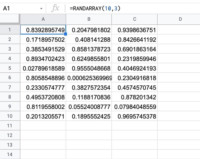
Here’s a RANDARRAY formula that generates an array of random numbers between 0 and 1, across 10 rows and 3 columns:
=RANDARRAY(10, 3)which gives an output:
🔗 The RANDARRAY template is available at the bottom of this article.
RANDARRAY Function Syntax
=RANDARRAY(rows, columns)It takes zero, one, or two arguments.
So RANDARRAY(), RANDARRAY(10), and RANDARRAY(5,5) are all valid formulas.
rows
The first argument is the number of rows to return. This is optional. If only one argument is supplied to the function, it determines the row count.
columns
The second argument is the number of columns to return. This is an optional argument. If omitted, it defaults to a value of 1.
RANDARRAY Function Examples
Firstly, RANDARRAY without any arguments generates a random number in a single cell, equivalent to the RAND function:
=RANDARRAY()RANDARRAY with a single argument generates random numbers in a column, e.g. this formula generates 5 random numbers in a vertical orientation:
=RANDARRAY(5)To generate a single row of random numbers, set the first argument to 1:
=RANDARRAY(1, 5)RANDARRRAY with two arguments generates random numbers across rows and columns, e.g. this formula generates random numbers across 10 rows and 5 columns:
=RANDARRAY(10, 5)RANDARRAY Function Notes
RANDARRAY is a volatile function, which means it recalculates every time your spreadsheet changes.
If you have a lot of RANDARRAY functions in your Sheet (or a lot of downstream formulas that reference a RANDARRAY function), then this can lead to slow Google Sheets because it will keep recalculating all those formulas with every change.
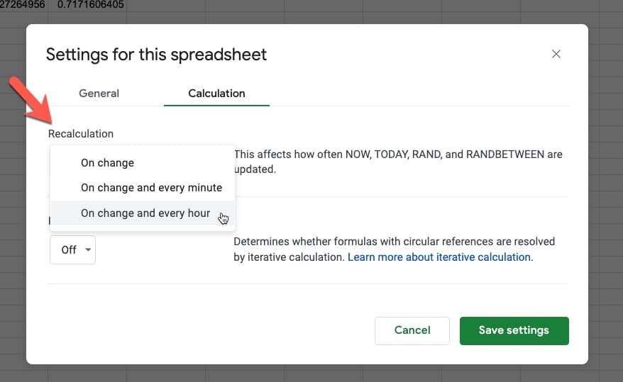
RANDARRAY can also be set to update hourly or even every minute.
Go to File > Settings > Calculation
Select the hour or minute options under the Recalculation dropdown menu:
See Also
To generate a single random number, use the RAND function.
To generate a random integer (whole number) between two values, use the RANDBETWEEN function.
Generate Random Whole Numbers With RANDARRAY
Use this array formula to generate an array of whole numbers between 1 and 10, across 10 rows and 5 columns:
=ArrayFormula(ROUND(RANDARRAY(10,5)*10))Similarly, to get values between 1 and 1000, use this formula:
=ArrayFormula(ROUND(RANDARRAY(10,5)*1000))Finally, to get an array of random whole numbers between two values, e.g. 250 and 700, use this formula:
=ArrayFormula(ROUND(RANDARRAY(10,5)*(700-250))+250)How To Sort A List Randomly Using A RANDARRAY Formula
RANDARRAY is useful for sorting lists randomly.
You assign each item in the list a random number between 0 and 1 and then sort those numbers in ascending order, which will randomize the order of the items.
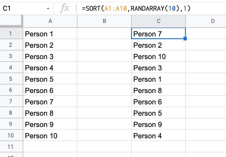
For example, suppose there are 10 names in column A.
This formula combines the SORT function and RANDARRAY function to randomize the order:
=SORT(A1:A10,RANDARRAY(10),1)The output is:
RANDARRAY Function Template
Click here to open a view-only copy >>
Feel free to make a copy: File > Make a copy…
If you can’t access the template, it might be because of your organization’s Google Workspace settings. If you right-click the link and open it in an Incognito window you’ll be able to see it.
It’s part of the Math family of functions in Google Sheets. You can read about it in the Google Documentation.
Is there a way to randomly enter values from a list. I want to make a squares spreadsheet that will randomly enter the titles across the top row and left-most column (think Jeopardy! style board).
Hi Phil,
Yes, you can use the SORT function with the RANDARRAY to sort lists randomly, which I think will achieve what you’re after.
Suppose you have headings in column A1:A4.
Use this formula to randomly sort that list:
=SORT(A1:A4,RANDARRAY(COUNTA(A1:A4)),1)And if you want it transposed for a header row, use this:
=TRANSPOSE(SORT(A1:A4,RANDARRAY(COUNTA(A1:A4)),1))Hope this helps!
Ben
Thanks for the help here. Is there a way to create an array of random whole numbers, with each row totaling n (or not surpassing a certain number), for example?
For example, I want a row (with 10 columns), and each cell has a random number (doesn’t have to be normally distributed), where the row SUM does not surpass a certain number. TIA!
There a lot of ways to achieve what you want, but they might not all match what you wish to achieve. You haven’t fully specified your requirements.
But if you want a list of (for example) 10 random numbers that sum to less than 100, the easiest way is to use Ben’s formula for a random array of whole numbers but limit them all to between zero and ten (or between zero and your desired total divided by the size of the row).
Eg., for 10 numbers and the total less than 100, try entering:
=ArrayFormula(ROUND(RANDARRAY(1,10)*10))
This matches what you have asked for, though it may not match what you actually wanted!
I have a list of agents with multiple tickets in Raw Data sheet, I want to select 5 tickets for every agent and paste it into another sheet. I created a list of unique agents and paste this at the side, but is not working.
=TRANSPOSE(SORT(FILTER(‘Raw Data’!C2:C, ‘Raw Data’!B2:B=A2),RANDARRAY(5)))
I want to take an array of numbers (10 columns, 20 rows) that is populated with numbers and randomize the rows and columns in both. For example, what is in a cell could end up in another column and in another row. If it was letters, the source could look like the randomized result.
SOURCE RESULT
a b c d g j a k
e f g h c l f d
i j k l b i h e
I just posted, but it did not keep the formatting of my example. There were 2 arrays of letters, each 4 columns and 3 rows.