The RANDBETWEEN function in Google Sheets is used to generate a random integer (whole number) between two values.
For example, this RANDBETWEEN formula generates a random number between 1 and 10:
=RANDBETWEEN(1,10)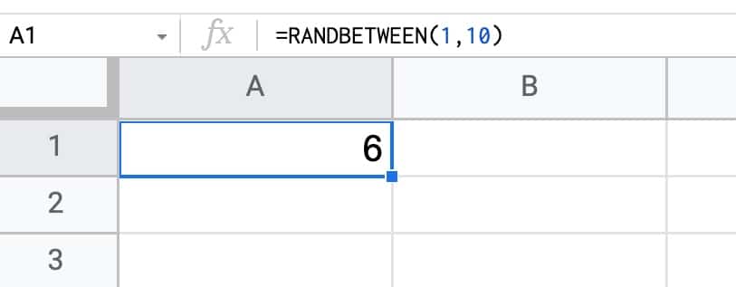
The function will generate a new random number each time your Sheet changes.
RANDBETWEEN Function Examples
This formula generates a random number between 1 and 1000:
=RANDBETWEEN(1,1000)To reference bounds in other cells, use this formula with your LOW value in A1 and your HIGH value in A2:
=RANDBETWEEN(A1,A2)Use the RANDBETWEEN function to generate negative numbers, for example between -100 and -1:
=RANDBETWEEN(-100,-1)This RANDBETWEEN formula generates a random number between -999 and 999:
=RANDBETWEEN(-999,999)🔗 Get these examples and others in the template at the bottom of this article.
RANDBETWEEN Function Syntax
=RANDBETWEEN(low, high)It takes two arguments:
low
An integer (whole number) that represents the lower bound of your random number set.
high
An integer (whole number) that represents the upper bound of your random number set.
RANDBETWEEN Notes
The RANDBETWEEN function is a volatile function, which means it recalculates every time a change is made in your Sheet or every time you open your Google Sheet.
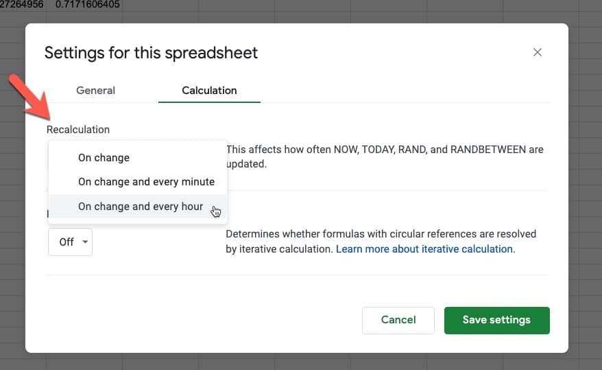
The RANDBETWEEN function can also be forced to recalculate every hour or every minute.
To force recalculations, go to the menu: File > Settings > Calculation
Select the hour or minute options under the Recalculation dropdown menu:
If you have a lot of RANDBETWEEN functions in your Sheet (or a lot of downstream formulas that reference a RANDBETWEEN function), this can lead to slow Google Sheets because it will keep recalculating all those formulas with every change.
If decimal numbers are used as input values, the LOW value will be rounded up for the lower boundary and the HIGH value will be rounded down for the upper boundary.
For example:
=RANDBETWEEN(2.5,3.5)will always output 3 because the LOW value of 2.5 equates to an integer of 3 as the lower random number bound, and the HIGH value of 3.5 equates to an integer of 3 too, as the upper random number bound.
See Also
To generate a random decimal number, use the RAND Function.
To generate an array of random numbers, use the RANDARRAY Function.
How To Select A Random Item From A Column Using RANDBETWEEN
Suppose we have data in column A and we want to select a random item from this list.
Use this formula, which combines the RANDBETWEEN function, the COUNTA function, and the INDEX function, to return a random item:
=INDEX(A2:A21,RANDBETWEEN(1,COUNTA(A2:A21)))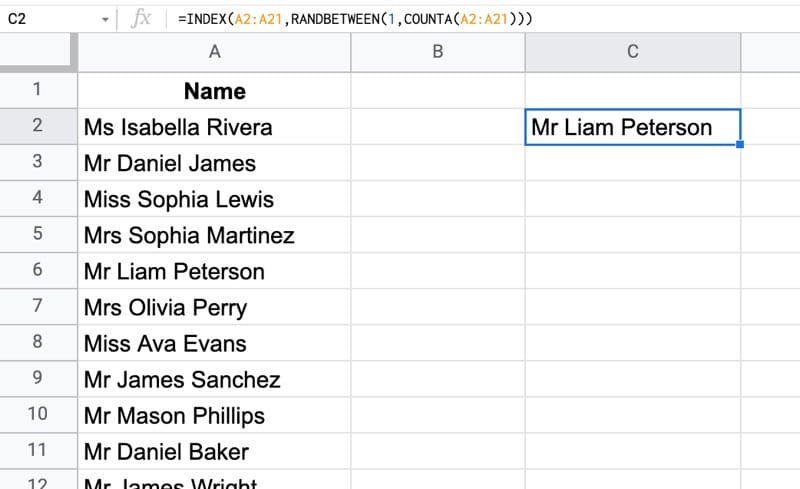
Let’s understand this formula by using the onion framework to break it down, starting from the innermost function:
=COUNTA(A2:A21)counts how many values we have in column A.
Then:
=RANDBETWEEN(1,COUNTA(A2:A21))generates a random number between 1 and the count of values in the range A2:A21.
Finally, the INDEX function returns the item from column A at the position denoted by the random number:
=INDEX(A2:A21,RANDBETWEEN(1,COUNTA(A2:A21)))RANDBETWEEN And CHOOSE Function
Combine the RANDBETWEEN function and the CHOOSE function to pick random items from a list:
=CHOOSE(RANDBETWEEN(1,5),"Person 1","Person 2","Person 3","Person 4","Person 5")The values can also be referenced in cells, as in this example:
=CHOOSE(RANDBETWEEN(1,5),A1,A2,A3,A4,A5)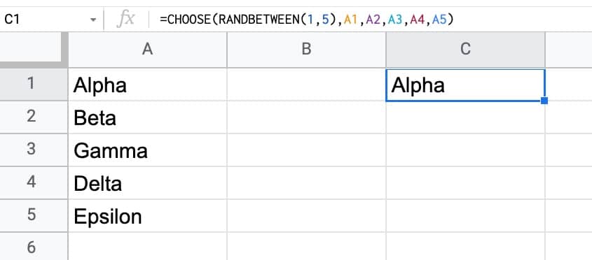
RANDBETWEEN Function Template
Click here to open a view-only copy >>
Feel free to make a copy: File > Make a copy…
If you can’t access the template, it might be because of your organization’s Google Workspace settings. If you right-click the link and open it in an Incognito window you’ll be able to see it.
It’s part of the Math family of functions in Google Sheets. You can read about it in the Google Documentation.